Feed: AWS Big Data Blog.

Toyota Motor Corporation (TMC), a global automotive manufacturer, has made “connected cars” a core priority as part of its broader transformation from an auto company to a mobility company. In recent years, TMC and its affiliate technology and big data company, Toyota Connected, have developed an array of new technologies to provide connected services that enhance customer safety and the vehicle ownership experience. Today, Toyota’s connected cars come standard with an on-board Data Communication Module (DCM) that links to a Controller Area Network (CAN). By using this hardware, Toyota provides various connected services to its customers.

Some of the connected services help drivers to safely enjoy their cars. Telemetry data is available from the car 24×7, and Toyota makes the data available to its dealers (when their customers opt-in for data sharing). For instance, a vehicle’s auxiliary battery voltage declines over time. With this data, dealership staff can proactively contact customers to recommend a charge prior to experiencing any issues. This automotive telemetry can also help fleet management companies monitor vehicle diagnostics, perform preventive maintenance and help avoid breakdowns.

There are other services such as usage-based auto insurance that leverage driving behavior data that can help safe drivers receive discounts on their car insurance. Telemetry plays a vital role in understanding driver behavior. If drivers choose to opt-in, a safety score can be generated based on their driving data and drivers can use their smartphones to check their safe driving scores.

A vehicle generates data every second, which can be bundled into larger packets at one-minute intervals. With millions of connected cars that have data points available every second, the incredible scale required to capture and store that data is immense—there are billions of messages daily generating petabytes of data. To make this vision a reality, Toyota Connected’s Mobility Team embarked on building a real-time “Toyota Connected Data Lake.” Given the scale, we leveraged AWS to build this platform. In this post, we show how we built the data lake and how we provide significant value to our customers.

Overview

The guiding principles for architecture and design that we used are as follows:

• Serverless: We want to use cloud native technologies and spend minimal time on infrastructure maintenance.
• Rapid speed to market: We work backwards from customer requirements and iterate frequently to develop minimally viable products (MVPs).
• Cost-efficient at scale.
• Low latency: near real time processing.

Our data lake needed to be able to:

• Capture and store new data (relational and non-relational) at petabyte scale in real time.
• Provide analytics that go beyond batch reporting and incorporate real time and predictive capabilities.
• Democratize access to data in a secure and governed way, allowing our team to unleash their creative energy and deliver innovative solutions.

The following diagram shows the high-level architecture

Walkthrough

We built the serverless data lake with Amazon S3 as the primary data store, given the scalability and high availability of S3. The entire process is automated, which reduces the likelihood of human error, increases efficiency, and ensures consistent configurations over time, as well as reduces the cost of operations.

The key components of a data lake include Ingest, Decode, Transform, Analyze, and Consume:

• Ingest: Connected vehicles send telemetry data once a minute—which includes speed, acceleration, turns, geo location, fuel level, and diagnostic error codes. This data is ingested into Amazon Kinesis Data Streams, processed through AWS Lambda to make it readable, and the “raw copy” is saved through Amazon Kinesis Data Firehose into an S3
• Decode:  Data arriving into the Kinesis data stream in the ‘Decode’ pillar is decoded by a serverless Lambda function, which does most of the heavy lifting. Based upon a proprietary specification, this Lambda function does the bit-by-bit decoding of the input message to capture the particular sensor values. The small input payload of 35KB with data from over 180 sensors is now decoded and converted to a JSON message of 3 MB. This is then compressed and written to the ‘Decoded S3 bucket’.
• Transform:  The aggregation jobs leverage the massively parallel capability of Amazon EMR, decrypt the decoded messages and convert the data to Apache Parquet Apache Parquet is a columnar storage file format designed for querying large amounts of data, regardless of the data processing framework, or programming language. Parquet allows for better compression, which reduces the amount of storage required. It also reduces I/O, since we can efficiently scan the data. The data sets are now available for analytics purposes, partitioned by masked identification numbers as well as by automotive models and dispatch type. A separate set of jobs transform the data and store it in Amazon DynamoDB to be consumed in real time from APIs.
• Consume: Applications needing to consume the data make API calls through the Amazon API Gateway. Authentication to the API calls is based on temporary tokens issued by Amazon Cognito.
• Analyze: Data analytics can be directly performed off Amazon S3 by leveraging serverless Amazon Athena. Data access is democratized and made available to data science groups, who build and test various models that provide value to our customers.

Additionally, comprehensive monitoring is set up by leveraging Amazon CloudWatch, Amazon ES, and AWS KMS for managing the keys securely.

Scalability

The scalability capabilities of the building blocks in our architecture that allow us to reach this massive scale are:

• S3: S3 is a massively scalable key-based object store that is well-suited for storing and retrieving large datasets. S3 partitions the index based on key name. To maximize performance of high-concurrency operations on S3, we introduced randomness into each of the Parquet object keys to increase the likelihood that the keys are distributed across many partitions.
• Lambda: We can run as many concurrent functions as needed and can raise limits as required with AWS support.
• Kinesis Firehose: It scales elastically based on volume without requiring any human intervention. We batch requests up to 128MiB or 15 minutes, whichever comes earlier to avoid small files. Additional details are available in Srikanth Kodali’s blog post.
• Kinesis Data Streams: We developed an automated program that adjusts the shards based on incoming volume. This is based on the Kinesis Scaling Utility from AWS Labs, which allows us to scale in a way similar to EC2 Auto Scaling groups.
• API Gateway: automatically scales to billions of requests and seamlessly handles our API traffic.
• EMR cluster: We can programmatically scale out to hundreds of nodes based on our volume and scale in after processing is completed.

Our volumes have increased seven-fold since we migrated to AWS and we have only adjusted the number of shards in Kinesis Data Streams and the number of core nodes for EMR processing to scale with the volume.

Security in the AWS cloud

AWS provides a robust suite of security services, allowing us to have a higher level of security in the AWS cloud. Consistent with our security guidelines, data is encrypted both in transit and at rest. Additionally, we use VPC Endpoints, allowing us to keep traffic within the AWS network.

Data protection in transit:

Data protection at rest:

• S3 server-side encryption handles all encryption, decryption and key management transparently. All user data stored in DynamoDB is fully encrypted at rest, for which we use an AWS-owned customer master key at no additional charge. Server-side encryption for Kinesis Data streams and Kinesis Data Firehose is also enabled to ensure that data is encrypted at rest.

Cost optimization

Given our very large data volumes, we were methodical about optimizing costs across all components of the infrastructure. The ultimate goal was to figure out the cost of the APIs we were exposing. We developed a robust cost model validated with performance testing at production volumes:

• NAT gateway: When we started this project, one of the significant cost drivers was traffic flowing from Lambda to Kinesis Data Firehose that went over the NAT gateway, since Kinesis Data Firehose did not have a VPC endpoint. Traffic flowing through the NAT gateway costs $0.045/GB, whereas traffic flowing through the VPC endpoint costs $0.01/GB. Based on a product feature request from Toyota, AWS implemented this feature (VPC Endpoint for Firehose) early this year. We implemented this feature, which resulted in a four-and-a-half-fold reduction in our costs for data transfer.
• Kinesis Data Firehose: Since Kinesis Data Firehose did not support encryption of data at rest initially, we had to use client-side encryption using KMS–this was the second significant cost driver. We requested a feature for native server-side encryption in Kinesis Data Firehose. This was released earlier this year and we enabled server-side encryption on the Kinesis Data Firehose stream. This removed the Key Management Service (KMS), resulting in another 10% reduction in our total costs.

Since Kinesis Data Firehose charges based on the amount of data ingested ($0.029/GB), our Lambda function compresses the data before writing to Kinesis Data Firehose, which saves on the ingestion cost.

• S3– We use lifecycle policies to move data from S3 (which costs $0.023/GB) to Amazon S3 Glacier (which costs $0.004/GB) after a specified duration. Glacier provides a six-fold cost reduction over S3. We further plan to move the data from Glacier to Amazon S3 Glacier Deep Archive (which costs $0.00099/GB), which will provide us a four-fold reduction over Glacier costs. Additionally, we have set up automated deletes of certain data sets at periodic intervals.
• EMR– We were planning to use AWS Glue and keep the architecture serverless, but made the decision to leverage EMR from a cost perspective. We leveraged spot instances for transformation jobs in EMR, which can provide up to 60% savings. The hourly jobs complete successfully with spot instances, however the nightly aggregation jobs leveraging r5.4xlarge instances failed frequently as sufficient spot capacity was not available. We decided to move to “on-demand” instances, while we finalize our strategy for “reserved instances” to reduce costs.
• DynamoDB: Time to Live (TTL) for DynamoDB lets us define when items in a table expire so that they can be automatically deleted from the database. We enabled TTL to expire objects that are not needed after a certain duration. We plan to use reserved capacity for read and write control units to reduce costs. We also use DynamoDB auto scaling ,which helps us manage capacity efficiently, and lower the cost of our workloads because they have a predictable traffic pattern. In Q2 of 2019, DynamoDBremoved the associated costs of DynamoDB Streams used in replicating data globally, which translated to extra cost savings in global tables.

• Amazon DynamoDB Accelerator(DAX):  Our DynamoDB tables are front-ended by DAX, which improves the response time of our application by dramatically reducing read latency, as compared to using DynamoDB. Using DAX, we also lower the cost of DynamoDB by reducing the amount of provisioned read throughput needed for read-heavy applications.
• Lambda: We ran benchmarks to arrive at the optimal memory configuration for Lambda functions. Memory allocation in Lambda determines CPU allocation and for some of our Lambda functions, we allocated higher memory, which results in faster execution, thereby reducing the amount of GB-seconds per function execution, which saves time and cost. Using DynamoDB Accelerator (DAX) from  Lambda has several benefits for serverless applications that also use DynamoDB. DAX can improve the response time of your application by dramatically reducing read latency, as compared to using DynamoDB. For serverless applications, combining Lambda with DAX provides an additional benefit: Lower latency results in shorter execution times, which means lower costs for Lambda.
• Kinesis Data Streams: We scale our streams through an automated job, since our traffic patterns are fairly predictable. During peak hours we add additional shards and delete them during the off-peak hours, thus allowing us to reduce costs when shards are not in use

Enhancing customer safety

The Data Lake presents multiple opportunities to enhance customer safety. Early detection of market defects and pinpointing of target vehicles affected by those defects is made possible through the telemetry data ingested from the vehicles. This early detection leads to early resolution way before the customer is affected. On-board software in the automobiles can be constantly updated over-the-air (OTA), thereby saving time and costs. The automobile can generate a Health Check Report based on the driving style of its drivers, which can create the ideal maintenance plan for drivers for worry-free driving.

The driving data for an individual driver based on speed, sharp turns, rapid acceleration, and sudden braking can be converted into a “driver score” which ranges from 1 to 100 in value. The higher the driver-score, the safer the driver. Drivers can view their scores on mobile devices and monitor the specific locations of harsh driving on the journey map. They can then use this input to self-correct and modify their driving habits to improve their scores, which will not only result in a safer environment but drivers could also get lower insurance rates from insurance companies. This also gives parents an opportunity to monitor the scores for their teenage drivers and coach them appropriately on safe driving habits. Additionally, notifications can be generated if the teenage driver exceeds an agreed-upon speed or leaves a specific area.

Summary

The automated serverless data lake is a robust scalable platform that allows us to analyze data as it becomes available in real time. From an operations perspective, our costs are down significantly. Several aggregation jobs that took 15+ hours to run, now finish in 1/40th of the time. We are impressed with the reliability of the platform that we built. The architectural decision to go serverless has reduced operational burden and will also allow us to have a good handle on our costs going forward. Additionally, we can deploy this pipeline in other geographies with smaller volumes and only pay for what we consume.

Our team accomplished this ambitious development in a short span of six months. They worked in an agile, iterative fashion and continued to deliver robust MVPs to our business partners. Working with the service teams at AWS on product feature requests and seeing them come to fruition in a very short time frame has been a rewarding experience and we look forward to the continued partnership on additional requests.

About the Authors

Sandeep Kulkarni drives Cloud Strategy and Architecture for Fortune 500 companies. His passion is to accelerate digital transformation for customers and build highly scalable and cost-effective solutions in the cloud. In his spare time, he loves to do yoga and gardening.

Shravanthi Denthumdas is the director of mobility services at Toyota Connected.Her team is responsible for building the Data Lake and delivering services that allow drivers to safely enjoy their cars. In her spare time, she likes to spend time with her family and children.

Feed: James Serra’s Blog.
Author: James Serra.

I had a previous blog comparing Cosmos DB to a relational database (see Understanding Cosmos DB coming from a relational world) and one topic that it did not address that I want to now is how to handle reference tables that are common in the relational database world.

A big difference with Cosmos DB compared to a relational database is you will create a denormalized data model.  Take a person record for example.  You will embed all the information related to a person, such as their contact details and addresses, into a single JSON document.  Retrieving a complete person record from the database is now a single read operation against a single container and for a single item.  Updating a person record, with their contact details and addresses, is also a single write operation against a single item.  By denormalizing data, your application typically will have better read performance and write performance and allow for a scale-out architecture since you don’t need to join tables. 

(Side note: “container” is the generic term. Depending on the API, a specific term is used such as “collection” for the Cosmos DB API). Think of a container as one or more tables in the relational world. Going a little deeper, think of a container as a group of one or more “entities” which share the same partition key. A relational table shares a schema, but containers are not bound in that way.)

Embedding data works nicely for many cases but there are scenarios when denormalizing your data will cause more problems than it is worth.  In a document database, you can have information in one document that relates to data in other documents. While there may be some use cases that are better suited for a relational database than in Cosmos DB (see below), in most cases you can handle relationships in Cosmos DB by creating a normalized data model for them, with the tradeoff that it can require more round trips to the server to read data (but improve the efficiency of write operations since less data is written).  In general, use normalized data models to represent one-to-many relationships or many-to-many relationships when related data changes frequently. The key is knowing whether the cost of the updates is greater than the cost of the queries.

When using a normalized data model, your application will need to handle creating the reference document.  One way would be to use a change feed that triggers on the creation of a new document – the change feed essentially triggers an Azure function that creates the  relationship record.

When using a normalized data model, your application will need to query the multiple documents that need to be joined (costing more money because it will use more request units), and do the joining within the application (i.e. join a main document with documents that contain the reference data) as you cannot do a “join” between documents within different containers in Cosmos DB (joins between documents within the same container can be done via self-joins).  Since every time you display a document it needs to search the entire container for the name, it would be best to put the other document type (the reference data) in a different container so you can have different partition keys for each document type (read up on how partitioning can make a big impact on performance and cost).

Note that “partitioning” in a RDBMS compared to Cosmos DB are different things: partitioning in Cosmos DB refers to “sharding” or “horizontal partitioning“, where replica sets which contain both the data and copies of compute (database) resources operating in a “shared nothing” architecture (i.e. scaled “horizontally” where each compute resource (server node) operates independently of every other node, but with a programming model transparent to developers). Conversely, what is often referred to as “partitioning” in a RDBMS is purely a separation of data into separate file groups within a shared compute (database) environment. This is also often called “vertical partitioning”.

Another option that is common pattern for NoSQL databases is to create a separate container to satisfy specific queries.  For example, having a container for products based on category and another container for products based on geography.  Both of those containers for my query/app are being sourced from one that is my “main” or “source” container that is being updated (front end, or another app) and the change feed attached to that pushes out to my other containers that I use for my queries.  This means duplicating data, but storage is cheap and you save costs to retrieve data (think of those extra containers as covering indexes in the relational database world). 

Since joining data can involve multiple ways of reading the data, it’s important to understand the two ways to read data using the Azure Cosmos DB SQL API:

• Point reads – You can do a key/value lookup on a single item ID and partition key. The item ID and partition key combination is the key and the item itself is the value. For a 1 KB document, point reads typically cost 1 request unit with a latency under 10ms. Point reads return a single item
• SQL queries – You can query data by writing queries using the Structured Query Language (SQL) as a JSON query language. Queries always cost at least 2.3 request units and, in general, will have a higher and more variable latency than point reads. Queries can return many items. See Getting started with SQL queries

The key in deciding when to use a normalized data model is how frequently the data will change.  If the data only changes once a year it may not be worthwhile to create a reference document and instead just do an update to all the documents.  But be aware that the update has to be done from the client side spread over the affected documents, doing it in batches as one big UPDATE statement does not exist in Cosmos DB.  You will need to retrieve the entire document from Cosmos DB, update the property/properties in your application and then call the ‘Replace’ method in the Cosmos DB SDK to replace the document in question (see CosmosDb – Updating a Document (Partially)). If you are using SQL API and .NET or Java, you can consider using bulk support (.NET) or bulk executor (Java). Other ideas would involve using change feed, or if you really need a level of ACID consistency, you can achieve this using stored procedures, with snapshot isolation scoped to a single partition (this is not the same as stored procedures in SQL – rather these are designed specifically to support multi-doc transactions).  

Also be aware that because there is currently no concept of a constraint, foreign-key or otherwise, any inter-document relationships that you have in documents are effectively “weak links” and will not be verified by the database itself.  If you want to ensure that the data a document is referring to actually exists, then you need to do this in your application, or through the use of server-side triggers or stored procedures on Azure Cosmos DB.

What are OLTP scenarios where a relational database is essential?

Avoiding the broader topic of when to use a relational database over a non-relational database, there are a few use cases where a relational database is essential:

• The customer experience and comfort zone is with relational databases. It is a reality that relational databases are ahead in the maturity curve with respect to tooling (an example would be foreign-key constraint behavior). However, it should be noted that this is not the same as saying that “more use cases are technically better suited to the relational model”. Rather, the barrier to entry in new customer projects tends to be lower because mindshare is greater in the relational space. In these cases, it often isn’t worth the effort for companies to upskill
• The system really needs strict ACID semantics across the entire dataset. Sharded/partitioned databases like Cosmos DB will not provide ACID guarantees across the entire set of physical partitions (and likely never will). In reality, however, the use cases where this is necessary is quite small. Things like transaction management and other SDK-level things that go along with these aspects come easier in the RDBMS space, but this is really the same as above point – RDBMS is ahead on maturity curve for user-level tooling to help abstract paradigm specific concepts – but this does not make the paradigm better suited to a greater number of use cases
• Having a single data store that services both operational and analytical needs with equal utility, including tabular models – this is probably the most powerful argument, and NoSQL engines are likely never going to serve a data structure that coalesces as well into tabular models that produce reports, charts, graphs, etc. But again, history has proven that, at scale, the “one fits all” approach can have some non-trivial drawbacks. And the new Analytical Store in Cosmos DB is addressing the need to service both operational and analytical needs

You can create complex hierarchical “relationships” in Cosmos DB, which would have to be modelled in separate tables in an RDBMS. Cosmos DB can’t handle them using joins – but again, this is a paradigmatic/semantic difference, not a fundamental flaw in the database model itself. In order to do the equivalent of what one may be trying to achieve in a relational database, you may have to “unlearn what you have learned”, but this comes back to your comfort level with a RDBMS, which is not a trivial thing and can be the main and very valid reason for staying with a RDBMS.

In summary, in a NoSQL database like Cosmos DB, most use cases are covered. Some things are a little harder (due to lack of maturity in tooling), but most things are easier, many things can only be done in NoSQL (i.e. handling millions of transactions per second), and very few things cannot be done in a NoSQL database. Most NoSQL engines are characterized by having a lot more configurability, tunability, and flexibility than a RDBMS. And in many ways, that is the hardest challenge for newcomers.

More info:

Data modeling in Azure Cosmos DB

Video Data modelling and partitioning in Azure Cosmos DB: What every relational database user needs to know

Video A tour of Azure Cosmos DB database operations models

Feed: Planet MySQL
;
Author: Dave Stokes
;

     How does MySQL compare INTs with CHARs? I was asked this very question over the weekend and wanted to share that information plus some of the changes in MySQL 8.0.21 in this area.  And yes those changes are pretty big.

Casting

    Computers are good at making comparisons of two values but only if everything else the same.  Comparing an integer with another integer is simple.  Same data with same data type comparisons are a good thing.  But what about when you need to compare a numeric 7 with a “7” where the number is in a string?  In such cases one or both numbers need to be changed into the same basic data type. Imagine your favorite Harry Potter character waving their magic wand and shouting ‘accio data’ to change two different magical pieces of data into one common data type.  No, Hogwarts was the the reason this conversion is called casting but this ‘magic’ needs to be made for a good comparison.

    If you read the Optimizer Notes section of the MySQL 8.0.21 Release Notes you will run into a notice that MySQL injects casts to avoid mismatches for numeric and temporal data with string data. The big trick was keeping backward compatibility with previous versions while matching the SQL standard.  Now when the optimizer is comparing numeric and temporal types and the expected data type does not match  it will now add casting operations in the item tree inside expressions and conditions. For instance if you are comparing a YEAR to string they will both be converted to a DOUBLE.

Example

    We have two tables and are comparing an INT to a CHAR.  If we run EXPLAIN ANALYZE of the query we get the details.

*************************** 1. row ***************************

EXPLAIN: -> Inner hash join (cast(t2.k as double) = cast(t1.k as double))  (cost=4.75 rows=5) (actual time=1.759..1.771 rows=5 loops=1)

    -> Table scan on t1  (cost=0.22 rows=6) (actual time=1.670..1.677 rows=6 loops=1)

    -> Hash

        -> Table scan on t2  (cost=0.75 rows=5) (actual time=0.034..0.043 rows=5 loops=1)

    If we look at the original query we are trying to join two tables where the CHAR t2.k is equal to the INT t1.k.   The magenta highlighted text above shows where both the t2.k and the t1.k columns are cast as doubles.

    Running EXPLAIN without the ANALYZE we can see the query plan’s version of the query that has been generated by the optimizer.

    We can see that the original query of select * from t1 join t2 on t2.k = t1.k has been rewritten to select `demo`.`t1`.`id` AS `id`,`demo`.`t1`.`k` AS `k`,`demo`.`t2`.`id` AS `id`,`demo`.`t2`.`k` AS `k` from `demo`.`t1` join `demo`.`t2` where (cast(`demo`.`t2`.`k` as double) = cast(`demo`.`t1`.`k` as double)) by the optimizer.  

    I highly recommend looking at the query plan to help understand what the MySQL server needs to do to make your query work.  

Feed: Planet PostgreSQL.

In many PostgreSQL databases, you never have to think or worry about tuning autovacuum. It runs automatically in the background and cleans up without getting in your way.

But sometimes the default configuration is not good enough, and you have to tune autovacuum to make it work properly. This article presents some typical problem scenarios and describes what to do in these cases.

The many tasks of autovacuum

There are many autovacuum configuration parameters, which makes tuning complicated. The main reason is that autovacuum has many different tasks. In a way, autovacuum has to fix all the problems arising from PostgreSQL’s Multiversioning Concurrency Control (MVCC) implementation:

• clean up “dead tuples” left behind after UPDATE or DELETE operations
• update the free space map that keeps track of free space in table blocks
• update the visibility map that is required for index-only scans
• “freeze” table rows so that the transaction ID counter can safely wrap around
• schedule regular ANALYZE runs to keep the table statistics updated

Depending on which of these functionalities cause a problem, you need different approaches to tuning autovacuum.

Tuning autovacuum for dead tuple cleanup

The best-known autovacuum task is cleaning up of dead tuples from UPDATE or DELETE operations. If autovacuum cannot keep up with cleaning up dead tuples, you should follow these three tuning steps:

Make sure that nothing keeps autovacuum from reclaiming dead tuples

Check the known reasons that keep vacuum from removing dead tuples. Most often, the culprit are long running transactions. Unless you can remove these obstacles, tuning autovacuum will be useless.

If you cannot fight the problem at its root, you can use the configuration parameter idle_in_transaction_session_timeout to have PostgreSQL terminate sessions that stay “idle in transaction” for too long. That causes errors on the client side, but may be justified if you have no other way to keep your database operational. Similarly, to fight long-running queries, you can use statement_timeout.

Tuning autovacuum to run faster

If autovacuum cannot keep up with cleaning up dead tuples, the solution is to make it work faster. This may seem obvious, but many people fall into the trap of thinking that making autovacuum start earlier or run more often will solve the problem.

VACUUM is a resource-intensive operation, so autovacuum by default operates deliberately slowly. The goal is to have it work in the background without being in the way of normal database operation. But if your workload creates lots of dead tuples, you will have to make it more aggressive:

Setting autovacuum_vacuum_cost_delay to 0 will make autovacuum as fast as a manual VACUUM – that is, as fast as possible.

Since not all tables grow dead tuples at the same pace, it is usually best not to change the global setting in postgresql.conf, but to change the setting individually for busy tables:

ALTER TABLE busy_table SET (autovacuum_vacuum_cost_delay = 1);

Partitioning a table can also help with getting the job done faster; see below for more.

Change the workload so that fewer dead tuples are generated

If nothing else works, you have to see that fewer dead tuples are generated. Perhaps several UPDATEs to a single row could be combined to a single UPDATE?

Often you can significantly reduce the number of dead tuples by using “HOT updates”:

• set the fillfactor for the table to a value less than 100, so that INSERTs leave some free space in each block
• make sure that no column that you modify in the UPDATE is indexed

Then any SELECT or DML statement can clean up dead tuples, and there is less need for VACUUM.

Tuning autovacuum for index-only scans

The expensive part of an index scan is looking up the actual table rows. If all columns you want are in the index, it should not be necessary to visit the table at all. But in PostgreSQL you also have to check if a tuple is visible or not, and that information is only stored in the table.

To work around that, PostgreSQL has a “visibility map” for each table. If a table block is marked as “all visible” in the visibility map, you don’t have to visit the table for the visibility information.

So to get true index-only scans, autovacuum has to process the table and update the visibility map frequently. How you configure autovacuum for that depends on the kind of data modifications the query receives:

Tuning autovacuum for index-only scans on tables that receive UPDATEs or DELETEs

For that, you reduce autovacuum_vacuum_scale_factor for the table, for example

ALTER TABLE mytable SET (autovacuum_vacuum_scale_factor = 0.01);

It may be a good idea to also speed up autovacuum as described above.

Tuning autovacuum for index-only scans on tables that receive only INSERTs

This is simple from v13 on: tune autovacuum_vacuum_insert_scale_factor as shown above for autovacuum_vacuum_scale_factor.

For older PostgreSQL versions, the best you can do is to significantly lower autovacuum_freeze_max_age. The best value depends on the rate at which you consume transaction IDs. If you consume 100000 transaction IDs per day, and you want the table to be autovacuumed daily, you can set

ALTER TABLE insert_only SET (autovacuum_freeze_max_age = 100000);

To measure the rate of transaction ID consumption, use the function txid_current() (or pg_current_xact_id() from v13 on) twice with a longer time interval in between and take the difference.

Tuning autovacuum to avoid transaction wraparound problems

Normally, autovacuum takes care of that and starts a special “anti-warparound” autovacuum worker whenever the oldest transaction ID in a table is older than autovacuum_freeze_max_age transactions or the oldest multixact is older than autovacuum_multixact_freeze_max_age transactions.

Make sure than anti-wraparound vacuum can freeze tuples in all tables

Again, you have to make sure that there is nothing that blocks autovacuum from freezing old tuples and advancing pg_database.datfrozenxid and pg_database.datminmxid. Such blockers can be:

• very long running database sessions that keep a transaction open or have temporary tables (autovacuum cannot process temporary tables)
• data corruption, which can make all autovacuum workers fail with an error

To prevent data corruption, use good hardware and always run the latest PostgreSQL minor release.

Tuning tables that receive UPDATEs or DELETEs for anti-wraparound vacuum

On tables that receive UPDATEs or DELETEs, all that you have to do is to see that autovacuum is running fast enough to get done in time (see above).

Tuning tables that receive only INSERTs for anti-wraparound vacuum

From PostgreSQL v13 on, there are no special considerations in this case, because you get regular autovacuum runs on such tables as well.

Before that, insert-only tables were problematic: since there are no dead tuples, normal autovacuum runs are never triggered. Then, as soon as autovacuum_freeze_max_age or autovacuum_multixact_freeze_max_age are exceeded, you may suddenly get a massive autovacuum run that freezes a whole large table, takes a long time and causes massive I/O.

To avoid that, reduce autovacuum_freeze_max_age for such a table:

ALTER TABLE insert_only SET (autovacuum_freeze_max_age = 10000000);

Partitioning

With very big tables, it can be advisable to use partitioning. The advantage here is you can have several autovacuum workers working on several partitions in parallel, so that the partitioned table as a whole is done faster than a single autovacuum worker could.

If you have many partitions, you should increase autovacuum_max_workers, the maximum number of autovacuum workers.

Partitioning can also help with vacuuming tables that receive lots of updates, as long as the updates affect all partitions.

Tuning autoanalyze

Updating table statistics is a “side job” of autovacuum.

You know that automatic statistics collection does not happen often enough if your query plans get better after a manual ANALYZE of the table.

In that case, you can lower autovacuum_analyze_scale_factor so that autoanalyze processes the table more often:

ALTER TABLE mytable SET (autovacuum_analyze_scale_factor = 0.02);

An alternative is not to use the scale factor, but set autovacuum_analyze_threshold, so that table statistics are calculated whenever a fixed number of rows changes. For example, to configure a table to be analyzed whenever more than a million rows change:

ALTER TABLE mytable SET (
   autovacuum_analyze_scale_factor = 0,
   autovacuum_analyze_threshold = 1000000
);

Conclusion

Depending on your specific problem and your PostgreSQL version, there are different tuning knobs to make autovacuum do its job correctly. The many tasks of autovacuum and the many configuration parameters don’t make that any easier.

If the tips in this article are not enough for you, consider getting professional consulting.

Feed: Liquid Web.
Author: Ronald Caldwell
;

With much of our world shifting online in the past few months, reliable web hosting has become a critical business necessity. Whether you are hosting web sites, applications, or office infrastructure, it is vital to have the right plan with the right resources.

But how do you choose from the different types of web hosting?

Web hosting options abound and can be overwhelming for the average user.

There are undoubtedly many things to consider outside of the hosting choices themselves. Business owners need to consider budget, age of the project, third party software licenses (where applicable), and the list goes on.

Business owners need to evaluate their needs when it comes to specific web hosting offerings.

We seek to ease your stress by noting the different types of web hosting available and for whom they work best.

What are the Types of Web Hosting?

Shared Hosting

Shared hosting is web hosting where single sites get placed on a single server with other websites, all sharing RAM, CPU, storage, and bandwidth resources. These types of web hosting plans are typically the least expensive of the hosting options. Because of the sharing of resources across multiple websites, performance and security can also suffer.

For those just starting with a brand new site, shared hosting is a good starting point. The low cost is attractive but is only fit for static websites with not a lot of traffic. Businesses that aim to scale quickly should consider other hosting options with independent resources.

VPS Hosting

Virtual Private Server Hosting (VPS) is a dynamic virtualized hosting server within a parent server on cloud infrastructure. While many VPS servers can exist on the parent server, the resources get explicitly dedicated to the user, unlike shared hosting.

A cluster of servers makes up the cloud infrastructure behind VPS servers. The server instances themselves are independent partitions of the parent server with a set allocation of resources to each server instance.

They are single-tenant, which means the RAM, CPU cores, and storage is specific to a single user instead of being shared among many users.

A central feature of VPS hosting is root access. Users have full control of the environment and can carry out more configuration tweaks.

Liquid Web’s VPS Hosting offers all of this in upgradeable instances with packaged bandwidth. In addition to root-level access, users also get Secure Shell (SSH) and Secure File Transfer Protocol (SFTP) access. InterWorx, cPanel, and Plesk are the available control panels for Linux, and we offer Plesk for Windows servers.

A VPS solution is a great option if you are hosting a few websites and applications that are not resource-intensive. They are also the perfect solution for file storage and sharing.

Cloud Dedicated Hosting

Cloud Dedicated hosting is a single-instance dynamic virtualized hosting server on a parent server on cloud infrastructure. Both exist on the parent server, and the resources get explicitly dedicated to the user. The primary differentiation is the fact that a Cloud Dedicated server is the only server instance on the parent server.

Often called Hybrid Dedicated servers, Cloud Dedicated server hosting also gets backed by clustered cloud infrastructure.

Cloud Dedicated servers from Liquid Web provide options to fit the needs of business owners, Resellers, and agencies needing dedicated resources in an easily scalable virtual server. Whether you’re hosting resource-intensive websites and applications, multiple sites and apps, databases, or want simple upgrade options, Cloud Dedicated servers will work for you.

Dedicated Hosting

Dedicated hosting is a single-tenant environment where physical server hardware and resources belong to a single user. Primarily, the owner of the dedicated server operates off of the physical components with the operating system, web server stack, and optional control panel for their hosting environment.

Dedicated servers are popular among resellers and agencies hosting a large number of small websites and applications. They are also great for more significant sites and apps that need more resources.

Liquid Web has been in the industry for several years, offering Dedicated Hosting solutions. We have everything from smaller, single processor options to larger configurations with dual processors. And customizing your server hardware is easy to do with multiple options available from storage, RAM, chassis, and bandwidth.

Cloud Hosting

There are many implementations of cloud hosting environments. Cloud Hosting in general refers to a network infrastructure that includes multiple physical servers connected via software. Both the private and public clouds are forms of cloud hosting.

Private Cloud

Private Cloud hosting solution is a single-tenant environment. A single organization can take advantage of a cluster of servers in a private cloud environment and use the combined resources to fit their needs.

By leveraging software like VMware, businesses can create as many virtual machines as can be handled to run their SaaS applications, websites, or other projects. Liquid Web’s Private Cloud powered by VMWare and NetApp provides business owners and digital agencies a premier private cloud solution to stand up to today’s demands.

Public Cloud

On the other side of the spectrum from the private cloud is Public Cloud Hosting. Public cloud is a multi-tenant hosting environment where multiple organizations reside in the same hosting environment, siloed from one another.

It is elastic and scalable, much like a private cloud, but the infrastructure is not specific to one organization. The cluster is much more robust and managed by the provider, offering business owners the ability to deploy scalable solutions quickly. It is also more cost-effective than a private cloud since the provider removes the burden of organizations paying for an individual cluster.

Liquid Web is proud to bring our Cloud Servers solution to the masses. For customers looking to move their workload to the cloud and eliminate in-house hardware, this is the solution. Customers can reduce hardware costs for their websites and applications while gaining redundancy and high availability.

Specialized Hosting

Several other solutions exist within the realm of the above-mentioned hosting options. They are either built on top of, or combinations of, traditional or cloud solutions to create a complex infrastructure that meets your specific hosting needs.

Enterprise Hosting

Enterprise customers have needs that go beyond basic hosting. They deal with large amounts of traffic and need highly available solutions with no downtime. Disaster recovery is a must.

For Enterprise customers, Cloud Hosting is not always what they want. They often prefer dedicated infrastructure, running their sites and applications directly off of physical server hardware. They then duplicate it, and failover to another replicated setup should something happen to the production environment.

Liquid Web offers hosting for the Enterprise, including dedicated server clusters, high-performance setups equipped with load balancing, and high availability environments with failover.

HIPAA Compliant Hosting

HIPAA Compliant Hosting is dedicated hosting secured behind lock and key that can only be accessed by specific users with logs maintained, and specific processes followed to ensure data integrity and security at all times.

For business owners dealing with Protected Health Information (PHI) or Electronic Protected Health Information (ePHI), it is essential to have hosting that meets HIPAA requirements. The fines for loss or compromise of PHI can be steep, so it is imperative to ensure proper implementation of HIPAA hosting.

An independent auditing firm validated and confirmed that our data centers are compliant with HIPAA security and privacy guidelines. Their findings include administrative, physical, and technical safeguard measures.

Liquid Web has HIPAA Compliant dedicated server packages specific to the needs of those hosting PHI and ePHI. Speak with a hosting advisor today to ensure that you have the right solution and the information you need to get your HIPAA environment set up.

How Do I Choose Which Type of Web Hosting is Right for Me?

With the plethora of web hosting options available, how do you choose which hosting is right for your business? Keep the following guidelines in mind as you make your choice:

• Choose VPS Hosting if you are hosting a few websites and applications that are not resource-intensive.
• Choose Cloud Dedicated Hosting if you are hosting resource-intensive websites and applications, multiple sites and apps, databases, or want simple upgrade options.
• Choose Dedicated Hosting if you are a reseller or agency hosting a large number of small websites and applications or have significant sites and apps that need more resources. Also, choose this hosting option if you need more customizable storage options.
• Choose Private Cloud Hosting to leverage the cloud to create as many virtual machines as can be handled to run your SaaS applications, websites, or other projects.
• Choose Public Cloud Hosting if you are looking to move your workload to the cloud and eliminate in-house hardware. Also, choose this option to reduce hardware costs for your websites and applications while gaining redundancy and high availability.
• Choose Enterprise Hosting for complex needs requiring dedicated server clusters, high-performance setups equipped with load balancing, and high availability environments with failover.

Ready to get started? Speak with a hosting advisor today to set up the hosting environment that’s right for you.

Feed: Planet PostgreSQL.

Prometheus is a popular open source monitoring tool and we have many customers that leverage it when using the Crunchy  PostgreSQL Operator or Crunchy PostgreSQL High Availability. Prometheus ships out-of-the-box with its own time series data store but we’re big fans of Postgres, and we know Postgres can do time series just fine. Furthermore, if you’re already running PostgreSQL and using Prometheus to monitor it, why not just store that data in a Postgres database?

Just because you can do something, doesn’t mean you should, but in this case it’s not such a bad idea. By storing Prometheus metric data natively in Postgres we can leverage many of the other features of PostgreSQL including:

To make it easier for anyone that wants to use Postgres as their backing store for Prometheus, we’re proud to announce the release of the PostgreSQL Prometheus Adapter.

Prometheus + Postgres

Prometheus, a Cloud Native Computing Foundation project, is a systems and service monitoring system. It collects metrics from configured targets at given intervals, evaluates rule expressions, displays the results, and can trigger alerts if some condition is observed to be true.

Postgres is already a powerful, open source object-relational database system with over 20 years of active development and known for its  reliability, feature robustness, and performance.

PostgreSQL 12, released in 2019, brought major enhancements to its partitioning functionality, with an eye towards time-series data. The improvements include:

• Partitioning performance enhancements, including improved query performance on tables with thousands of partitions, improved insertion performance with INSERT and COPY, and the ability to execute ALTER TABLE ATTACH PARTITION without blocking queries
• Improved performance of many operations on partitioned tables
• Allows tables with thousands of child partitions to be processed efficiently by operations that only affect a small number of partitions
• Improve speed of COPY into partitioned tables

These time series improvements make it a great candidate to back our Prometheus monitoring setup.

Prometheus Storage Adapter

The Prometheus remote storage adapter concept allows for the storage of Prometheus time series data externally using a remote write protocol. This externally stored time series data can be read using remote read protocol.

For Prometheus to use PostgreSQL as remote storage, the adapter must implement a write method. This method will be called by Prometheus when storing data.

func (c *Client) Write(samples model.Samples) error {
   ...
}

For Prometheus to read remotely stored, the adapter must also implement a read method. This method will be called by Prometheus clients requesting data.

func (c *Client) Read(req *prompb.ReadRequest) (*prompb.ReadResponse, error) 
{
   ...
}

PostgreSQL Prometheus Adapter

PostgreSQL Prometheus Adapter is a remote storage adapter designed to utilize PostgreSQL 12 native partitioning enhancements to efficiently store Prometheus time series data in a PostgreSQL database.

The PostgreSQL Prometheus Adapter design is based on partitioning and threads. Incoming data is processed by one or more threads and one or more writer threads will store data in PostgreSQL daily or hourly partitions. Partitions will be auto-created by the adapter based on the timestamp of incoming data.

Let’s build our PostgreSQL Prometheus Adapter setup

git clone https://github.com/CrunchyData/postgresql-prometheus-adapter.git

cd postgresql-prometheus-adapter
make

cd postgresql-prometheus-adapter
make container

You can also tweak a number of settings for the adapter as well. To get a look at all the settings you can configure:

./postgresql-prometheus-adapter --help
usage: postgresql-prometheus-adapter []

Remote storage adapter [ PostgreSQL ]

Flags:
  -h, --help                           Show context-sensitive help (also try --help-long and --help-man).
      --adapter-send-timeout=30s       The timeout to use when sending samples to the remote storage.
      --web-listen-address=":9201"     Address to listen on for web endpoints.
      --web-telemetry-path="/metrics"  Address to listen on for web endpoints.
      --log.level=info                 Only log messages with the given severity or above. One of: [debug, info, warn, error]
      --log.format=logfmt              Output format of log messages. One of: [logfmt, json]
      --pg-partition="hourly"          daily or hourly partitions, default: hourly
      --pg-commit-secs=15              Write data to database every N seconds
      --pg-commit-rows=20000           Write data to database every N Rows
      --pg-threads=1                   Writer DB threads to run 1-10
      --parser-threads=5               parser threads to run per DB writer 1-10

Depending on your metric counts, we’d recommend configuring:

• –parser-threads – this controls how many threads will be started to process incoming data
• –pg-partition – control whether to use hourly or daily partitions
• –pg-threads – controls how many database writer threads will be started to insert data in database

Putting it all together

First we’re going to configure out Prometheus setup to have our remote write and read endpoints. To do this edit your prometheus.yml and then restart your Prometheus:

remote_write:
    - url: "http://:9201/write"
remote_read:
    - url: "http://:9201/read"

Next we’re going to set the environment variable for our database, start the adapter.

export DATABASE_URL="postgres://username:password@host:5432/database"
cd postgresql-prometheus-adapter
./postgresql-prometheus-adapter

If you’re running everything inside a container you setup will look a bit different:

podman run --rm  
  --name postgresql-prometheus-adapter  
  -p 9201:9201 
  -e DATABASE_URL="postgres://username:password@host:5432/database"  
  --detach 
  crunchydata/postgresql-prometheus-adapterl:latest

The following environment settings can be passed to podman for tweaking adapter settings:

adapter_send_timeout=30s       The timeout to use when sending samples to the remote storage.
web_listen_address=":9201"     Address to listen on for web endpoints.
web_telemetry_path="/metrics"  Address to listen on for web endpoints.
log_level=info                 Only log messages with the given severity or above. One of: [debug, info, warn, error]
log_format=logfmt              Output format of log messages. One of: [logfmt, json]
pg_partition="hourly"          daily or hourly partitions, default: hourly
pg_commit_secs=15              Write data to database every N seconds
pg_commit_rows=20000           Write data to database every N Rows
pg_threads=1                   Writer DB threads to run 1-10
parser_threads=5               parser threads to run per DB writer 1-10

How do I test the adapter without running a Prometheus instance ?

You can simulate the Prometheus interface using: 

Avalanche supports load testing for services accepting data via Prometheus remote_write API.

./avalanche 
  --remote-url="http://:9201/write" 
  --metric-count=10 
  --label-count=15 
  --series-count=30 
  --remote-requests-count=100 
  --remote-write-interval=100ms

Feel free to tweak the above settings based on your test case.

Further Reading

Crunchy High Availability PostgreSQL provides an integrated high availability solution for enterprises with “always on” data requirements . This solution provides performance requirements, high availability, load balancing, and scalability.

Give our Prometheus Postgres adapter a try today or visit PostgreSQL Prometheus Adapter to read more about it and how to utilize this adapter.

Feed: AWS Big Data Blog.

Customers use Amazon Redshift for everything from accelerating existing database environments, to ingesting weblogs for big data analytics. Amazon Redshift is a fully managed, petabyte-scale, massively parallel data warehouse that offers simple operations and high performance. Amazon Redshift provides an open standard JDBC/ODBC driver interface, which allows you to connect your existing business intelligence (BI) tools and reuse existing analytics queries.

Amazon Redshift can run any type of data model, from a production transaction system third-normal-form model to star and snowflake schemas, data vault, or simple flat tables.

This post takes you through the most common performance-related opportunities when adopting Amazon Redshift and gives you concrete guidance on how to optimize each one.

What’s new

This post refreshes the Top 10 post from early 2019. We’re pleased to share the advances we’ve made since then, and want to highlight a few key points.

Query throughput is more important than query concurrency.

Configuring concurrency, like memory management, can be relegated to Amazon Redshift’s internal ML models through Automatic WLM with Query Priorities. On production clusters across the fleet, we see the automated process assigning a much higher number of active statements for certain workloads, while a lower number for other types of use-cases. This is done to maximize throughput, a measure of how much work the Amazon Redshift cluster can do over a period of time. Examples are 300 queries a minute, or 1,500 SQL statements an hour. It’s recommended to focus on increasing throughput over concurrency, because throughput is the metric with much more direct impact on the cluster’s users.

In addition to the optimized Automatic WLM settings to maximize throughput, the concurrency scaling functionality in Amazon Redshift extends the throughput capability of the cluster to up to 10 times greater than what’s delivered with the original cluster. The tenfold increase is a current soft limit, you can reach out to your account team to increase it.

Investing in the Amazon Redshift driver.

AWS now recommends the Amazon Redshift JDBC or ODBC driver for improved performance. Each driver has optional configurations to further tune it for higher or lower number of statements, with either fewer or greater row counts in the result set.

Ease of use by automating all the common DBA tasks.

In 2018, the SET DW “backronym” summarized the key considerations to drive performance (sort key, encoding, table maintenance, distribution, and workload management). Since then, Amazon Redshift has added automation to inform 100% of SET DW, absorbed table maintenance into the service’s (and no longer the user’s) responsibility, and enhanced out-of-the-box performance with smarter default settings. Amazon Redshift Advisor continuously monitors the cluster for additional optimization opportunities, even if the mission of a table changes over time. AWS publishes the benchmark used to quantify Amazon Redshift performance, so anyone can reproduce the results.

Scaling compute separately from storage with RA3 nodes and Amazon Redshift Spectrum.

Although the convenient cluster building blocks of the Dense Compute and Dense Storage nodes continue to be available, you now have a variety of tools to further scale compute and storage separately. Amazon Redshift Managed Storage (the RA3 node family) allows for focusing on using the right amount of compute, without worrying about sizing for storage. Concurrency scaling lets you specify entire additional clusters of compute to be applied dynamically as-needed. Amazon Redshift Spectrum uses the functionally-infinite capacity of Amazon Simple Storage Service (Amazon S3) to support an on-demand compute layer up to 10 times the power of the main cluster, and is now bolstered with materialized view support.

Pause and resume feature to optimize cost of environments

All Amazon Redshift clusters can use the pause and resume feature. For clusters created using On Demand, the per-second grain billing is stopped when the cluster is paused. Reserved Instance clusters can use the pause and resume feature to define access times or freeze a dataset at a point in time.

Tip #1: Precomputing results with Amazon Redshift materializes views

Materialized views can significantly boost query performance for repeated and predictable analytical workloads such as dash-boarding, queries from BI tools, and extract, load, transform (ELT) data processing. Data engineers can easily create and maintain efficient data-processing pipelines with materialized views while seamlessly extending the performance benefits to data analysts and BI tools.

Materialized views are especially useful for queries that are predictable and repeated over and over. Instead of performing resource-intensive queries on large tables, applications can query the pre-computed data stored in the materialized view.

When the data in the base tables changes, you refresh the materialized view by issuing the Amazon Redshift SQL statement “refresh materialized view“. After issuing a refresh statement, your materialized view contains the same data as a regular view. Refreshes can be incremental or full refreshes (recompute). When possible, Amazon Redshift incrementally refreshes data that changed in the base tables since the materialized view was last refreshed.

To demonstrate how it works, we can create an example schema to store sales information, each sale transaction and details about the store where the sales took place.

To view the total amount of sales per city, we create a materialized view with the create materialized view SQL statement (city_sales) joining records from two tables and aggregating sales amount (sum(sales.amount)) per city (group by city):

CREATE MATERIALIZED VIEW city_sales AS 
  (
  SELECT st.city, SUM(sa.amount) as total_sales
  FROM sales sa, store st
  WHERE sa.store_id = st.id
  GROUP BY st.city
  );

Now we can query the materialized view just like a regular view or table and issue statements like “SELECT city, total_sales FROM city_sales” to get the following results. The join between the two tables and the aggregate (sum and group by) are already computed, resulting in significantly less data to scan.

When the data in the underlying base tables changes, the materialized view doesn’t automatically reflect those changes. You can refresh the data stored in the materialized view on demand with the latest changes from the base tables using the SQL refresh materialized view command. For example, see the following code:

!-- let's add a row in the sales base table

INSERT INTO sales (id, item, store_id, customer_id, amount) 
VALUES(8, 'Gaming PC Super ProXXL', 1, 1, 3000);

SELECT city, total_sales FROM city_sales WHERE city = 'Paris'

|city |total_sales|
|-----|-----------|
|Paris|        690|

!-- the new sale is not taken into account !!
-- let's refresh the materialized view
REFRESH MATERIALIZED VIEW city_sales;

SELECT city, total_sales FROM city_sales WHERE city = 'Paris'

|city |total_sales|
|-----|-----------|
|Paris|       3690|

!-- now the view has the latest sales data

The full code for this use case is available as a very simple demo is available as a gist in GitHub.

You can also extend the benefits of materialized views to external data in your Amazon S3 data lake and federated data sources. With materialized views, you can easily store and manage the pre-computed results of a SELECT statement referencing both external tables and Amazon Redshift tables. Subsequent queries referencing the materialized views run much faster because they use the pre-computed results stored in Amazon Redshift, instead of accessing the external tables. This also helps you reduce the associated costs of repeatedly accessing the external data sources, because you can only access them when you explicitly refresh the materialized views.

Tip #2: Handling bursts of workload with concurrency scaling and elastic resize

The legacy, on-premises model requires you to estimate what the system will need 3-4 years in the future to make sure you’re leasing enough horsepower at the time of purchase. But the ability to resize a cluster allows for right-sizing your resources as you go. Amazon Redshift extends this ability with elastic resize and concurrency scaling.

Elastic resize lets you quickly increase or decrease the number of compute nodes, doubling or halving the original cluster’s node count, or even change the node type. You can expand the cluster to provide additional processing power to accommodate an expected increase in workload, such as Black Friday for internet shopping, or a championship game for a team’s web business. Choose classic resize when you’re resizing to a configuration that isn’t available through elastic resize. Classic resize is slower but allows you to change the node type or expand beyond the doubling or halving size limitations of an elastic resize. 

Elastic resize completes in minutes and doesn’t require a cluster restart. For anticipated workload spikes that occur on a predictable schedule, you can automate the resize operation using the elastic resize scheduler feature on the Amazon Redshift console, the AWS Command Line Interface (AWS CLI), or API.

Concurrency scaling allows your Amazon Redshift cluster to add capacity dynamically in response to the workload arriving at the cluster.

By default, concurrency scaling is disabled, and you can enable it for any workload management (WLM) queue to scale to a virtually unlimited number of concurrent queries, with consistently fast query performance. You can control the maximum number of concurrency scaling clusters allowed by setting the “max_concurrency_scaling_clusters” parameter value from 1 (default) to 10 (contact support to raise this soft limit). The free billing credits provided for concurrency scaling is often enough and the majority of customers using this feature don’t end up paying extra for it. For more information about the concurrency scaling billing model see Concurrency Scaling pricing.

You can monitor and control the concurrency scaling usage and cost by creating daily, weekly, or monthly usage limits and instruct Amazon Redshift to automatically take action (such as logging, alerting or disabling further usage) if those limits are reached. For more information, see Managing usage limits in Amazon Redshift.

Together, these options open up new ways to right-size the platform to meet demand. Before these options, you needed to size your WLM queue, or even an entire Amazon Redshift cluster, beforehand in anticipation of upcoming peaks.

Tip #3: Using the Amazon Redshift Advisor to minimize administrative work

Amazon Redshift Advisor offers recommendations specific to your Amazon Redshift cluster to help you improve its performance and decrease operating costs.

Advisor bases its recommendations on observations regarding performance statistics or operations data. Advisor develops observations by running tests on your clusters to determine if a test value is within a specified range. If the test result is outside of that range, Advisor generates an observation for your cluster. At the same time, Advisor creates a recommendation about how to bring the observed value back into the best-practice range. Advisor only displays recommendations that can have a significant impact on performance and operations. When Advisor determines that a recommendation has been addressed, it removes it from your recommendation list. In this section, we share some examples of Advisor recommendations:

Distribution key recommendation

Advisor analyzes your cluster’s workload to identify the most appropriate distribution key for the tables that can significantly benefit from a KEY distribution style. Advisor provides ALTER TABLE statements that alter the DISTSTYLE and DISTKEY of a table based on its analysis. To realize a significant performance benefit, make sure to implement all SQL statements within a recommendation group.

The following screenshot shows recommendations regarding distribution keys.

If you don’t see a recommendation, that doesn’t necessarily mean that the current distribution styles are the most appropriate. Advisor doesn’t provide recommendations when there isn’t enough data or the expected benefit of redistribution is small.

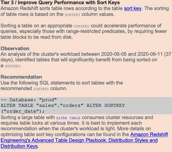
Sort key recommendation

Sorting a table on an appropriate sort key can accelerate query performance, especially queries with range-restricted predicates, by requiring fewer table blocks to be read from disk.

Advisor analyzes your cluster’s workload over several days to identify a beneficial sort key for your tables. See the following screenshot.

If you don’t see a recommendation for a table, that doesn’t necessarily mean that the current configuration is the best. Advisor doesn’t provide recommendations when there isn’t enough data or the expected benefit of sorting is small.

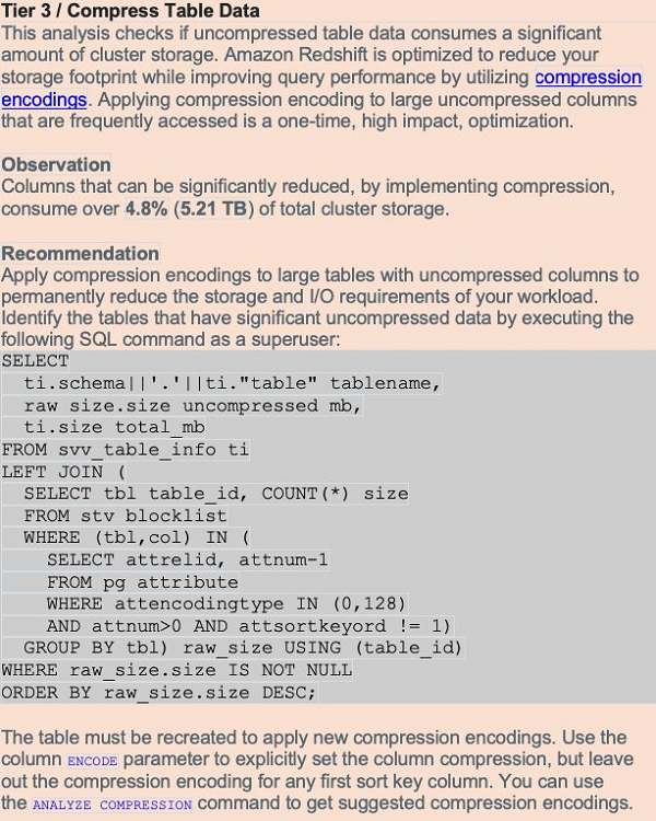
Table compression recommendation

Amazon Redshift is optimized to reduce your storage footprint and improve query performance by using compression encodings. When you don’t use compression, data consumes additional space and requires additional disk I/O. Applying compression to large uncompressed columns can have a big impact on your cluster.

The compression analysis in Advisor tracks uncompressed storage allocated to permanent user tables. It reviews storage metadata associated with large uncompressed columns that aren’t sort key columns.

The following screenshot shows an example of table compression recommendation.

Table statistics recommendation

Maintaining current statistics helps complex queries run in the shortest possible time. The Advisor analysis tracks tables whose statistics are out-of-date or missing. It reviews table access metadata associated with complex queries. If tables that are frequently accessed with complex patterns are missing statistics, Amazon Redshift Advisor creates a critical recommendation to run ANALYZE. If tables that are frequently accessed with complex patterns have out-of-date statistics, Advisor creates a suggested recommendation to run ANALYZE.

The following screenshot shows a table statistics recommendation.

Tip #4: Using Auto WLM with priorities to increase throughput

Auto WLM simplifies workload management and maximizes query throughput by using ML to dynamically manage memory and concurrency, which ensures optimal utilization of the cluster resources

Amazon Redshift runs queries using the queuing system (WLM). You can define up to eight queues to separate workloads from each other.

Amazon Redshift Advisor automatically analyzes the current WLM usage and can make recommendations to get more throughput from your cluster. Periodically reviewing the suggestions from Advisor helps you get the best performance.

Query priorities is a feature of Auto WLM that lets you assign priority ranks to different user groups or query groups, to ensure that higher priority workloads get more resources for consistent query performance, even during busy times. It is a good practice to set up query monitoring rules (QMR) to monitor and manage resource intensive or runaway queries. QMR also enables you to dynamically change a query’s priority based on its runtime performance and metrics-based rules you define.

For more information on migrating from manual to automatic WLM with query priorities, see Modifying the WLM configuration.

It’s recommended to take advantage of Amazon Redshift’s short query acceleration (SQA). SQA uses ML to run short-running jobs in their own queue. This keeps small jobs processing, rather than waiting behind longer-running SQL statements. SQA is enabled by default in the default parameter group and for all new parameter groups. You can enable and disable SQA via a check box on the Amazon Redshift console, or by using the Amazon Redshift CLI.

If you enable concurrency scaling, Amazon Redshift can automatically and quickly provision additional clusters should your workload begin to back up. This is an important consideration when deciding the cluster’s WLM configuration.

A common pattern is to optimize the WLM configuration to run most SQL statements without the assistance of supplemental memory, reserving additional processing power for short jobs. Some queueing is acceptable because additional clusters spin up if your needs suddenly expand. To enable concurrency scaling on a WLM queue, set the concurrency scaling mode value to AUTO. You can best inform your decisions by reviewing the concurrency scaling billing model. You can also monitor and control the concurrency scaling usage and cost by using the Amazon Redshift usage limit feature.

In some cases, unless you enable concurrency scaling for the queue, the user or query’s assigned queue may be busy, and you must wait for a queue slot to open. During this time, the system isn’t running the query at all. If this becomes a frequent problem, you may have to increase concurrency.

First, determine if any queries are queuing, using the queuing_queries.sql admin script. Review the maximum concurrency that your cluster needed in the past with wlm_apex.sql, or get an hour-by-hour historical analysis with wlm_apex_hourly.sql. Keep in mind that increasing concurrency allows more queries to run, but each query gets a smaller share of the memory. You may find that by increasing concurrency, some queries must use temporary disk storage to complete, which is also sub-optimal.

Tip #5: Taking advantage of Amazon Redshift data lake integration

Amazon Redshift is tightly integrated with other AWS-native services such as Amazon S3 which let’s the Amazon Redshift cluster interact with the data lake in several useful ways.

Amazon Redshift Spectrum lets you query data directly from files on Amazon S3 through an independent, elastically sized compute layer. Use these patterns independently or apply them together to offload work to the Amazon Redshift Spectrum compute layer, quickly create a transformed or aggregated dataset, or eliminate entire steps in a traditional ETL process.

• Use the Amazon Redshift Spectrum compute layer to offload workloads from the main cluster, and apply more processing power to the specific SQL statement. Amazon Redshift Spectrum automatically assigns compute power up to approximately 10 times the processing power of the main cluster. This may be an effective way to quickly process large transform or aggregate jobs.
• Skip the load in an ELT process and run the transform directly against data on Amazon S3. You can run transform logic against partitioned, columnar data on Amazon S3 with an INSERT … SELECT statement. It’s easier than going through the extra work of loading a staging dataset, joining it to other tables, and running a transform against it.
• Use Amazon Redshift Spectrum to run queries as the data lands in Amazon S3, rather than adding a step to load the data onto the main cluster. This allows for real-time analytics.
• Land the output of a staging or transformation cluster on Amazon S3 in a partitioned, columnar format. The main or reporting cluster can either query from that Amazon S3 dataset directly or load it via an INSERT … SELECT statement.

Within Amazon Redshift itself, you can export the data into the data lake with the UNLOAD command, or by writing to external tables. Both options export SQL statement output to Amazon S3 in a massively parallel fashion. You can do the following:

• Using familiar CREATE EXTERNAL TABLE AS SELECT and INSERT INTO SQL commands, create and populate external tables on Amazon S3 for subsequent use by Amazon Redshift or other services participating in the data lake without the need to manually maintain partitions. Materialized views can also cover external tables, further enhancing the accessibility and utility of the data lake.
• Using the UNLOAD command, Amazon Redshift can export SQL statement output to Amazon S3 in a massively parallel fashion. This technique greatly improves the export performance and lessens the impact of running the data through the leader node. You can compress the exported data on its way off the Amazon Redshift cluster. As the size of the output grows, so does the benefit of using this feature. For writing columnar data to the data lake, UNLOAD can write partition-aware Parquet data.

Tip #6: Improving the efficiency of temporary tables

Amazon Redshift provides temporary tables, which act like normal tables but have a lifetime of a single SQL session. The proper use of temporary tables can significantly improve performance of some ETL operations. Unlike regular permanent tables, data changes made to temporary tables don’t trigger automatic incremental backups to Amazon S3, and they don’t require synchronous block mirroring to store a redundant copy of data on a different compute node. Due to these reasons, data ingestion on temporary tables involves reduced overhead and performs much faster. For transient storage needs like staging tables, temporary tables are ideal.

You can create temporary tables using the CREATE TEMPORARY TABLE syntax, or by issuing a SELECT … INTO #TEMP_TABLE query. The CREATE TABLE statement gives you complete control over the definition of the temporary table. The SELECT … INTO and C(T)TAS commands use the input data to determine column names, sizes and data types, and use default storage properties. Consider default storage properties carefully, because they may cause problems. By default, for temporary tables, Amazon Redshift applies EVEN table distribution with no column encoding (such as RAW compression) for all columns. This data structure is sub-optimal for many types of queries.

If you employ the SELECT…INTO syntax, you can’t set the column encoding, column distribution, or sort keys. The CREATE TABLE AS (CTAS) syntax instead lets you specify a distribution style and sort keys, and Amazon Redshift automatically applies LZO encoding for everything other than sort keys, Booleans, reals, and doubles. You can exert additional control by using the CREATE TABLE syntax rather than CTAS.

If you create temporary tables, remember to convert all SELECT…INTO syntax into the CREATE statement. This ensures that your temporary tables have column encodings and don’t cause distribution errors within your workflow. For example, you may want to convert a statement using this syntax:

SELECT column_a, column_b INTO #my_temp_table FROM my_table;

You need to analyze the temporary table for optimal column encoding:

Master=# analyze compression #my_temp_table;
Table | Column | Encoding
----------------+----------+---------
#my_temp_table | columb_a | lzo
#my_temp_table | columb_b | bytedict
(2 rows)

You can then convert the SELECT INTO a statement to the following:

BEGIN;

CREATE TEMPORARY TABLE my_temp_table(
column_a varchar(128) encode lzo,
column_b char(4) encode bytedict)
distkey (column_a) -- Assuming you intend to join this table on column_a
sortkey (column_b) -- Assuming you are sorting or grouping by column_b
;

INSERT INTO my_temp_table SELECT column_a, column_b FROM my_table;

COMMIT;

If you create a temporary staging table by using a CREATE TABLE LIKE statement, the staging table inherits the distribution key, sort keys, and column encodings from the parent target table. In this case, merge operations that join the staging and target tables on the same distribution key performs faster because the joining rows are collocated. To verify that the query uses a collocated join, run the query with EXPLAIN and check for DS_DIST_NONE on all the joins.

You may also want to analyze statistics on the temporary table, especially when you use it as a join table for subsequent queries. See the following code:

ANALYZE my_temp_table;

With this trick, you retain the functionality of temporary tables but control data placement on the cluster through distribution key assignment. You also take advantage of the columnar nature of Amazon Redshift by using column encoding.

Tip #7: Using QMR and Amazon CloudWatch metrics to drive additional performance improvements

In addition to the Amazon Redshift Advisor recommendations, you can get performance insights through other channels.

The Amazon Redshift cluster continuously and automatically collects query monitoring rules metrics, whether you institute any rules on the cluster or not. This convenient mechanism lets you view attributes like the following:

• The CPU time for a SQL statement (query_cpu_time)
• The amount of temporary space a job might ‘spill to disk’ (query_temp_blocks_to_disk)
• The ratio of the highest number of blocks read over the average (io_skew)

It also makes Amazon Redshift Spectrum metrics available, such as the number of Amazon Redshift Spectrum rows and MBs scanned by a query (spectrum_scan_row_count and spectrum_scan_size_mb, respectively). The Amazon Redshift system view SVL_QUERY_METRICS_SUMMARY shows the maximum values of metrics for completed queries, and STL_QUERY_METRICS and STV_QUERY_METRICS carry the information at 1-second intervals for the completed and running queries respectively.

The Amazon Redshift CloudWatch metrics are data points for use with Amazon CloudWatch monitoring. These can be cluster-wide metrics, such as health status or read/write, IOPS, latency, or throughput. It also offers compute node–level data, such as network transmit/receive throughput and read/write latency. At the WLM queue grain, there are the number of queries completed per second, queue length, and others. CloudWatch facilitates monitoring concurrency scaling usage with the metrics ConcurrencyScalingSeconds and ConcurrencyScalingActiveClusters.

It’s recommended to consider the CloudWatch metrics (and the existing notification infrastructure built around them) before investing time in creating something new. Similarly, the QMR metrics cover most metric use cases and likely eliminate the need to write custom metrics.

Tip #8: Federated queries connect the OLAP, OLTP and data lake worlds

The new Federated Query feature in Amazon Redshift allows you to run analytics directly against live data residing on your OLTP source system databases and Amazon S3 data lake, without the overhead of performing ETL and ingesting source data into Amazon Redshift tables. This feature gives you a convenient and efficient option for providing realtime data visibility on operational reports, as an alternative to micro-ETL batch ingestion of realtime data into the data warehouse. By combining historical trend data from the data warehouse with live developing trends from the source systems, you can gather valuable insights to drive real-time business decision making.

For example, consider sales data residing in three different data stores:

• Live sales order data stored on an Amazon RDS for PostgreSQL database (represented as “ext_postgres” in the following external schema)
• Historical sales data warehoused in a local Amazon Redshift database (represented as “local_dwh”)
• Archived, “cold” sales data older than 5 years stored on Amazon S3 (represented as “ext_spectrum”)

We can create a late binding view in Amazon Redshift that allows you to merge and query data from all three sources. See the following code:

CREATE VIEW store_sales_integrated AS 
SELECT * FROM ext_postgres.store_sales_live 
UNION ALL 
SELECT * FROM local_dwh.store_sales_current 
UNION ALL 
SELECT ss_sold_date_sk, ss_sold_time_sk, ss_item_sk, ss_customer_sk, ss_cdemo_sk, 
ss_hdemo_sk, ss_addr_sk, ss_store_sk, ss_promo_sk, ss_ticket_number, ss_quantity, 
ss_wholesale_cost, ss_list_price, ss_sales_price, ss_ext_discount_amt, 
ss_ext_sales_price, ss_ext_wholesale_cost, ss_ext_list_price, ss_ext_tax, 
ss_coupon_amt, ss_net_paid, ss_net_paid_inc_tax, ss_net_profit 
FROM ext_spectrum.store_sales_historical 
WITH NO SCHEMA BINDING
;

Currently, direct federated querying is supported for data stored in Amazon Aurora PostgreSQL and Amazon RDS for PostgreSQL databases, with support for other major RDS engines coming soon. You can also use the federated query feature to simplify the ETL and data-ingestion process. Instead of staging data on Amazon S3, and performing a COPY operation, federated queries allow you to ingest data directly into an Amazon Redshift table in one step, as part of a federated CTAS/INSERT SQL query.

For example, the following code shows an upsert/merge operation in which the COPY operation from Amazon S3 to Amazon Redshift is replaced with a federated query sourced directly from PostgreSQL:

BEGIN;

CREATE TEMP TABLE staging (LIKE ods.store_sales);

-- replace the following COPY from S3: 
   /*COPY staging FROM 's3://yourETLbucket/daily_store_sales/' 
   IAM_ROLE 'arn:aws:iam::<account_id>:role/<s3_reader_role>' 
   DELIMITER '|' COMPUPDATE OFF; */
      
-- with this federated query to load staging data directly from PostgreSQL source
INSERT INTO staging SELECT * FROM pg.store_sales p
    WHERE p.last_updated_date > (SELECT MAX(last_updated_date) FROM ods.store_sales);

DELETE FROM ods.store_sales USING staging s WHERE ods.store_sales.id = s.id;

INSERT INTO ods.store_sales SELECT * FROM staging;

DROP TABLE staging;

COMMIT;

For more information about setting up the preceding federated queries, see Build a Simplified ETL and Live Data Query Solution using Redshift Federated Query. For additional tips and best practices on federated queries, see Best practices for Amazon Redshift Federated Query.

Tip #9: Maintaining efficient data loads

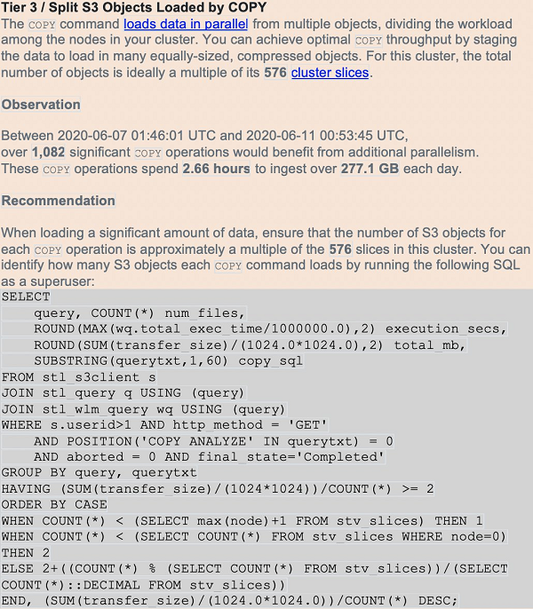
Amazon Redshift best practices suggest using the COPY command to perform data loads of file-based data. Single-row INSERTs are an anti-pattern. The COPY operation uses all the compute nodes in your cluster to load data in parallel, from sources such as Amazon S3, Amazon DynamoDB, Amazon EMR HDFS file systems, or any SSH connection.

When performing data loads, compress the data files whenever possible. For row-oriented (CSV) data, Amazon Redshift supports both GZIP and LZO compression. It’s more efficient to load a large number of small files than one large one, and the ideal file count is a multiple of the cluster’s total slice count. Columnar data, such as Parquet and ORC, is also supported. You can achieve best performance when the compressed files are between 1MB-1GB each.

The number of slices per node depends on the cluster’s node size (and potentially elastic resize history). By ensuring an equal number of files per slice, you know that the COPY command evenly uses cluster resources and complete as quickly as possible. Query for the cluster’s current slice count with SELECT COUNT(*) AS number_of_slices FROM stv_slices;.

Another script in the amazon-redshift-utils GitHub repo, CopyPerformance, calculates statistics for each load. Amazon Redshift Advisor also warns of missing compression or too few files based on the number of slices (see the following screenshot):

Conducting COPY operations efficiently reduces the time to results for downstream users, and minimizes the cluster resources utilized to perform the load.

Tip #10: Using the latest Amazon Redshift drivers from AWS

Because Amazon Redshift is based on PostgreSQL, we previously recommended using JDBC4 PostgreSQL driver version 8.4.703 and psql ODBC version 9.x drivers. If you’re currently using those drivers, we recommend moving to the new Amazon Redshift–specific drivers. For more information about drivers and configuring connections, see JDBC and ODBC drivers for Amazon Redshift in the Amazon Redshift Cluster Management Guide.

While rarely necessary, the Amazon Redshift drivers do permit some parameter tuning that may be useful in some circumstances. Downstream third-party applications often have their own best practices for driver tuning that may lead to additional performance gains.

For JDBC, consider the following:

• To avoid client-side out-of-memory errors when retrieving large data sets using JDBC, you can enable your client to fetch data in batches by setting the JDBC fetch size parameter or BlockingRowsMode.
• Amazon Redshift doesn’t recognize the JDBC maxRows parameter. Instead, specify a LIMIT clause to restrict the result set. You can also use an OFFSET clause to skip to a specific starting point in the result set.

For ODBC, consider the following:

• A cursor is enabled on the cluster’s leader node when useDelareFecth is enabled. The cursor fetches up to fetchsize/cursorsize and then waits to fetch more rows when the application request more rows.
• The CURSOR command is an explicit directive that the application uses to manipulate cursor behavior on the leader node. Unlike the JDBC driver, the ODBC driver doesn’t have a BlockingRowsMode mechanism.

It’s recommended that you do not undertake driver tuning unless you have a clear need. AWS Support is available to help on this topic as well.

Conclusion

Amazon Redshift is a powerful, fully managed data warehouse that can offer increased performance and lower cost in the cloud. As Amazon Redshift grows based on the feedback from its tens of thousands of active customers world-wide, it continues to become easier to use and extend its price-for-performance value proposition. Staying abreast of these improvements can help you get more value (with less effort) from this core AWS service.

We hope you learned a great deal about making the most of your Amazon Redshift account with the resources in this post.

If you have questions or suggestions, please leave a comment.

About the Authors

Matt Scaer is a Principal Data Warehousing Specialist Solution Architect, with over 20 years of data warehousing experience, with 11+ years at both AWS and Amazon.com.

Manish Vazirani is an Analytics Specialist Solutions Architect at Amazon Web Services.

Tarun Chaudhary is an Analytics Specialist Solutions Architect at AWS.

Feed: AWS Partner Network (APN) Blog.
Author: Oren Reuveni.

By Oren Reuveni, Sr. Partner Solutions Architect – AWS SaaS Factory

Software-as-a-service (SaaS) products frequently use agents to gather data, execute actions, communicate with remote components, and run other product-related tasks in remote environments. These agents can be deployed in multiple forms and for multiple purposes.

If you manage multi-tenant SaaS environments and use agents, you face some unique challenges. Implementing such a solution requires adequate design.

For instance, you have to be sure those agents are securely identified and associated with their tenants, and that they are successfully isolated from accessing the data outside their context. The ability to configure tenant-related settings, such as tier type, and apply specific configuration changes can also be a challenge.

This post focuses on the deployment and management of agents in a SaaS environment. I will review the key considerations to keep in mind when building such solutions, and discuss the main challenges associated with registering a new agent in the system. I will also explore managing agents throughout their lifecycle in a multi-tenant SaaS environment.

In a follow-up post, I will demonstrate the concept described here using solution based on AWS IoT Core managed service.

About SaaS Agents

SaaS solutions agents are essentially logic that runs remotely in the customer’s environment that can be used to gather essential data, or execute actions on behalf of the SaaS application.

For example, an agent can send different metrics back to the SaaS environment, or run product-related tasks in the environment it’s deployed in. Let’s explore the concept by reviewing several key aspects.

Figure 1 – SaaS agents in a multi-tenant cloud environment.

Figure 1 depicts a scenario of managing multiple agents. The agents belong to different tenants.

In this stage, they are already registered in, and being managed by, a single SaaS environment. It’s critical for the SaaS provider to ensure each agent operates only within its scope, since these agents will be communicating with one shared, multi-tenant environment.

Two aspects of the SaaS agent model are key: registration and management. To register the agent, use the SaaS solution to generate credentials and registration data that enables the agent to establish a secure communication channel with the SaaS environment.

After you have registered the agent, the SaaS solution manages it throughout its lifecycle. This includes facilitating communication, ingestion of telemetry data, ongoing management of the agents, configuring and updating them, and disabling them if needed.

Challenges of Using Agents in a SaaS Environment

The introduction of agents into your SaaS model adds a new set of considerations to your application design and architecture. Agents add new dimensions to your solution footprint that can influence the security and performance of tenant environments.

Following is a list of key areas to keep in mind when using agents as part of a SaaS solution:

• Identity — Each agent has to be positively identified and correlated to its tenant. Security, activity metering, and service tiers are directly related to the agent’s identity.
• Isolation — The agent has to operate only within the scope of the tenant it belongs to, and cannot access another tenant’s data.
• Throttling and noisy neighbor mitigation — Since each tenant is sending and receiving data from their agents while using a shared environment, consider how or whether that data could introduce a noisy neighbor condition where one tenant’s impacts the experience of other tenants.
• Tenant management and configuration — Each tenant has to be managed and configured according to the customer’s requirements and contracted level of service. This point is strongly connected to automation.
• Automation — Automation reduces friction and that reduction is essential to agility. It can enable customers to set up agents using a self-service model or, in some cases, provide agent installation as a fully automated process during the onboarding stage. Your solution needs to support all phases of the agent’s lifecycle, including onboarding, management, and deletion.

This enables the SaaS provider to meet customer requirements and operate at larger scale.

Registering Agents

The first stage in working with agents is deploying them in their target environment and registering them with the SaaS solution. Registration ensures the agent:

1. Is identified by the system and associated with the right tenant.
2. Interacts with the tenant using the appropriate credentials and tenant scope.

While the SaaS provider designs and facilitates the agent registration process, the user is the entity that executes it in a self-service manner. The SaaS provider should make sure the agents are successfully going through the registration process, while ensuring they are coupled to the tenant they belong to, and that tenant data and configuration remain isolated.

As a first step, the agent’s installation package needs to be deployed in the target environment.

An agent can take several forms. It can be a code library or a binary deployed in a server. It can also be packaged as an AWS Lambda function, a container, or a server image like an Amazon Machine Image (AMI).

You can use different methods to deploy the agent. One common method is using an infrastructure as code tool such as AWS CloudFormation or Terraform. Another is using a script to automate deployment.

Figure 2 – Agent registration process.

After the agent is deployed in the target environment, provide it with registration data so it can authenticate and integrate with the SaaS environment. This data is generated in a self-service manner by the SaaS application user, interactively via the user interface, or programmatically via an API.

Communication with the agent needs to be secured, and you can do that in multiple ways. A common method is using a certificate to encrypt and sign the communication between the agent and SaaS environment. I will demonstrate the use of such a mechanism in the second part of this post.

Following is a possible format for such a token and registration data. Please note the token will most likely be encoded and encrypted prior to sending it over the wire.

This token is in JSON format:

{"registration_token_example": {
    "version": "v2.1",
    "timestamp": "VALUE",
    "registration_data": {
        "agent_id": "5he9f03h6btmjp07gjes",
        "tenant_id": "69c5ygydn2",
        "api_endpoint_to_contact": "https://ENDPOINT-NAME.execute-api.us-east-2.amazonaws.com",
        "path": "/register",
        "region": "eu-west-1"
    }
}}

Now, you can start the registration process. According to the suggested flow, the agent will be given this token as an argument when launched for the first time. This process mainly happens as a part of an automation for a single agent or multiple agents registration, but can be also executed manually by the SaaS solution user.

Once the agent has the token, it contacts the SaaS environment API endpoint and uses the chosen secure communication mechanism in order to authenticate. After the authentication phase completes, the data in the token is validated and processed to register it in the system.

As noted above, the agent’s token may contain the tenant identification data along with a unique ID that identifies the agent in the system. An alternative option is not sending this data at all, by using a unique identifier for the agent, and mapping it to the rest of the required data that will be stored on the SaaS environment side.

On the SaaS environment side, relevant elements like the agent’s profile and permissions are defined by the system according to the tenant it belongs to. As part of the implementation of this process, configuration data and tenant-specific data (like user defined scripts or other configuration parameters) can be also sent to the agent during the on-boarding stage.

At this point, the agent has the ability communicate with the SaaS environment and vice versa.

Managing Agents Throughout Their Lifecycle

An agent lifecycle begins with the registration process, and continues through ongoing management, monitoring, versioning, and deployment of updates. It usually ends with removing the agent from the system. To manage agents effectively, you must be able to handle version upgrades, deploy configuration changes, and aggregate the data they send.

Backwards compatibility is also a requirement since different agents can have different versions and configurations.

In agent-based environments, it’s often important for SaaS providers to seamlessly deploy new versions. Automating these updates allows you to avoid downtime, deliver better value for your customers, and better scale your operation.

Deploying a new version to thousands or even millions of agents must be automated because human operators delivering this task would take more time than is financially viable, and might produce errors. Carefully document the upgrade so you can handle potential errors, bugs, and deployment rollbacks, if necessary.

As your agents evolve, you’ll want to ensure you have mechanisms in place to accurately track the version history your agent. This is especially important since your system may support multiple versions of an agent at a given moment in time. Knowing the history of each version is essential to troubleshooting the various agents that could be deployed.

Data flow is another important topic to keep in mind. The agent can ship multiple types of data into the SaaS environment. It can be solution telemetry data (event log, for example), agent log data, or data that’s part of the product itself. The data that comes from the agents should be ingested automatically. It’s common for this data to be transformed and enriched prior to storing it in the system.

An example of that is splitting the data into per tenant partitions, or keeping different data types (say, logs and product-related data) in different data stores.

Agents may also need to support a way to surface alerts and notifications. A notification mechanism provides valuable information, such as agent usage metrics, to the user, or allows the SaaS provider to be informed about certain events like registration of a new agent. This allows the SaaS provider to have better insight into tenant activity patterns by sending notifications about tenant events and analyzing them.

Alerts (that are defined with thresholds) can set off alarms to notify the SaaS provider of unusual activity, or trigger mitigation mechanisms, such as scaling and tenant activity throttling.

The lifecycle usually ends when a managed environment becomes deprecated, or, for example, when a user decides to stop using the solution. Either case results in the need to delete the agent from the system. Another relevant scenario for ending the lifecycle is quickly disabling access to the system for rogue agents which, for example, can reside in an environment that was compromised or whose performance was impacted.

Conclusion

I have suggested a conceptual approach of how to register and manage the agents throughout their lifecycle. I talked about key topics to look into when building such solutions, reviewed the registration and onboarding flow, and discussed actions that are required during the ongoing work with the agents.

For SaaS environments that rely on agents, it’s essential to examine all the moving parts of the agent lifecycle. The goal here is to introduce agents without undermining the agility, security, or manageability of your SaaS environment. This means focusing on introducing all the mechanisms that ensure you can effectively deploy and manage your agents in a way that mitigates the friction they might introduce into your environment.

In a future post, I will use an example based on AWS IoT Core that implements the concept described here.

Learn More About AWS SaaS Factory

We encourage AWS Partner Network (APN) Technology Partners to reach out to their APN representative to inquire about working with the AWS SaaS Factory team. You can access additional technical and business best practices on the AWS SaaS Factory website.

ISVs that are not APN Partners can subscribe to the SaaS on AWS email list to receive updates about upcoming events, content launches, and program offerings.

Feed: MemSQL Blog.
Author: Amy Qiu.

You run a database. You try to anticipate the future. You try to provide sufficient, even generous, resources to accommodate future growth in your service. But sometimes, growth far exceeds even your most optimistic expectations, and now you have to figure out how to accommodate that. 

One obvious way of increasing your database’s ability to handle and service more data is to simply add more machines to your cluster. That should increase the number of cores, and the amounts of memory and disk space available in your cluster. But with a limited number of partitions, at some point, adding the number of cores and memory and disk won’t be able to increase the  parallelism and breadth of your database. 

Since partitions cannot span leaves, you cannot share data storage and processing between N leaves unless you have at least N partitions. Additionally, parallel query performance will be best when we have one or two cores per partition.   

Therefore, it would seem that being able to increase the number of partitions amongst which the data is spread out is critical for the cluster’s scalability. Until now, however, there has not been an easy and convenient way to do this in MemSQL. 

Introducing Backup with Split Partitions

In order to split the number of partitions in your database, we’ve come up with a clever strategy that adds partition splitting to the work of a backup operation. Normally, a full backup will create one backup for each partition database, with a .backup file for the snapshots of the rowstore portion of data, and a .backup_columns_num_tar file, or files, for the columnstore blobs of a partition. There is also rowstore backup for the reference database and a BACKUP_COMPLETE file for a completed backup. 

Figure 1. Normal backup – no split partitions

But for splitting partitions, each partition will actually generate backup files for two partitions – with each of these split partitions having the data required to create half of the original partition upon a restore. A multi-step hash function determines which of the new split partitions any row in the original partition should belong to, and this function splits all rows between the new split partitions in the backup. 

Figure 2. Backup with split partitions

We chose to piggyback on backup, because it was already a very sturdy and reliable operation that succeeds or fails very transparently and because backup already makes sure that we have a consistent image of the whole distributed database. 

When we restore our split backup, the split partitions in the backup will restore as split partitions in the cluster. 

Figure 3. Restore of backup with split partitions

As you can see, splitting partitions is actually a three-stage process consisting of taking a split backup, dropping the database, and restoring the split backup. Now let’s now see this in practice. 

Example Workflow

Pre-Split-Partitions Work 

(Optional) Add Leaves

If you’re expanding your database’s resources by adding new leaves, you will want to add the leaves first before taking a split backup. 

This could save you an extra step of rebalance partitions at the end of restore, since for all backups except for local filesystem backups, restore will start with creating partitions in a balanced way to begin with. An extra bonus is that recovery will be faster if recovery is spread out among more leaves and resources.

The command would look something like this:

ADD LEAF user[:'password']@'host'[:port] [INTO GROUP {1|2}]

The reason I recommend doing it before backup is because although you can add leaves anytime, if you were going to pause your workload for backup split, you would want to avoid any action like add leaves that would prolong your workload downtime. If you do end up adding leaves after restoring the split backup, or you did a backup with split partitions to a local filesystem location on each leaf, you will need to remember to run REBALANCE PARTITIONS after the restore completes .

(Optional, But Recommended) Pause Workload 

It is true for all backups that backups only contain writes up to the point of that backup. If you restore an old backup, you will not have new rows added after the old backup was taken. This holds true for our split backups as well. If you do not wish to lose any writes written after the split backup was taken, you should make sure that writes are blocked when the backup starts until the database is restored. 

Split Partitions Work

(Step 1) Backup with split partitions command:

BACKUP [DATABASE] db_name WITH SPLIT PARTITIONS TO [S3|AZURE] ‘backup_location’ [S3 or Azure configs and credentials]

Rowstore data will be split between the split backups, so the total size of rowstore split backups should be roughly the same as rowstore split backups. In your backup location, these will have the .backup postfix. Columnstore blobs of a partition will be duplicated between the split backups of that partition, and so columnstore blobs will take twice the disk space in a backup with split partitions. I recommend leaving enough space for two full backups in order to attempt one backup with split partitions. Once the split backups are restored and columnstore merger has run, the blobs will no longer be duplicated (more details in the optimize table portion below).

(Step 2) Normal drop database command:

DROP DATABASE db_name

If you have a disaster recovery database, drop the disaster recovery database at this time and recreate it after you’ve restored the database.

(Step 3) Normal restore database command:

RESTORE [DATABASE] db_name FROM [S3|AZURE] "backup_location" [S3 or Azure configs and credentials] 

Post-Split-Partitions Work 

(Optional, but Recommended) Unpause Workload

If you paused your write workload earlier, your workload can be unpaused as soon as restore runs. 

(Recommended) Explain Rebalance

If you backed up to NFS, S3 or Azure, and you did not add any leaves after you restored, there should be no rebalance work suggested the explain rebalance command. If you backed up to the local filesystem, which creates individual backups on every preexisting leaf and you have more leaves now, “explain rebalance” will most likely suggest a rebalance. 

(Optional, but Sometimes Recommended) Optimize Table

After the split database backups are restored, the background columnstore merger will automatically be triggered. So although backup with split partitions duplicated the columnstore blobs. The columnstore merger will eventually compact (and likely merge) the columnstore blobs so that they use less space on disk. After the merger is done, the database should get back to using roughly the same amount of disk space for the same amount of data as before the backup split, and all future normal backups will take a normal amount of space. Expect to see more CPU usage from this background process while it is reducing the disk usage of the blobs. 

After testing, we found that overly sparse segments incurred a performance hit for queries like    select and range queries. A performance-sensitive user may want to manually run optimize table on all the tables of the newly split database to explicitly trigger columnstore merger rather than waiting around for the background columnstore merger to eventually get to tidying up a particular table.  

Feed: AWS Big Data Blog.

Apache Hive is an open-source data warehouse package that runs on top of an Apache Hadoop cluster. You can use Hive for batch processing and large-scale data analysis. Hive uses Hive Query Language (HiveQL), which is similar to SQL.

ACID (atomicity, consistency, isolation, and durability) properties make sure that the transactions in a database are atomic, consistent, isolated, and reliable.

Amazon EMR 6.1.0 adds support for Hive ACID transactions so it complies with the ACID properties of a database. With this feature, you can run INSERT, UPDATE, DELETE, and MERGE operations in Hive managed tables with data in Amazon Simple Storage Service (Amazon S3). This is a key feature for use cases like streaming ingestion, data restatement, bulk updates using MERGE, and slowly changing dimensions.

This post demonstrates how to enable Hive ACID transactions in Amazon EMR, how to create a Hive transactional table, how it can achieve atomic and isolated operations, and the concepts, best practices, and limitations of using Hive ACID in Amazon EMR.

Enabling Hive ACID in Amazon EMR

To enable Hive ACID as the default for all Hive managed tables in an EMR 6.1.0 cluster, use the following hive-site configuration:

[
   {
      "classification": "hive-site",
      "properties": {
         "hive.support.concurrency": "true",
         "hive.exec.dynamic.partition.mode": "nonstrict",
         "hive.txn.manager": "org.apache.hadoop.hive.ql.lockmgr.DbTxnManager"
      }
   }
]

For the complete list of configuration parameters related to Hive ACID and descriptions of the preceding parameters, see Hive Transactions.

Hive ACID use case

In this section, we explain the Hive ACID transactions with a straightforward use case in Amazon EMR.

Enter the following Hive command in the master node of an EMR cluster (6.1.0 release) and replace <s3-bucket-name> with the bucket name in your account:

hive --hivevar location=<s3-bucket-name> -f s3://aws-bigdata-blog/artifacts/hive-acid-blog/hive_acid_example.hql 

After Hive ACID is enabled on an Amazon EMR cluster, you can run the CREATE TABLE DDLs for Hive transaction tables.

To define a Hive table as transactional, set the table property transactional=true.

The following CREATE TABLE DDL is used in the script that creates a Hive transaction table acid_tbl:

CREATE TABLE acid_tbl (key INT, value STRING, action STRING)
PARTITIONED BY (trans_date DATE)
CLUSTERED BY (key) INTO 3 BUCKETS
STORED AS ORC
LOCATION 's3://${hivevar:location}/acid_tbl' 
TBLPROPERTIES ('transactional'='true');

This script generates three partitions in the provided Amazon S3 path. See the following screenshot.

The first partition, trans_date=2020-08-01, has the data generated as a result of sample INSERT, UPDATE, DELETE, and MERGE statements. We use the second and third partitions when explaining minor and major compactions later in this post.

ACID is achieved in Apache Hive using three types of files: base, delta, and delete_delta. Edits are written in delta and delete_delta files.

The base file is created by the Insert Overwrite Table query or as the result of major compaction over a partition, where all the files are consolidated into a single base_<write id> file, where the write ID is allocated by the Hive transaction manager for every write. This helps achieve isolation of Hive write queries and enables them to run in parallel.

The INSERT operation creates a new delta_<write id>_<write id> directory.

The DELETE operation creates a new delete_delta_<write id>_<write id> directory.

To support deletes, a unique row__id is added to each row on writes. When a DELETE statement runs, the corresponding row__id gets added to the delete_delta_<write id>_<write id> directory, which should be ignored on reads. See the following screenshot.

The UPDATE operation creates a new delta_<write id>_<write id> directory and a delete<write id>_<write id> directory.

The following screenshot shows the second partition in Amazon S3, trans_date=2020-08-02.

A Hive transaction provides snapshot isolation for reads. When an application or query reads the transaction table, it opens all the files of a partition/bucket and returns the records from the last transaction committed.

Hive compactions

With the previously mentioned logic for Hive writes on a transactional table, many small delta and delete_delta files are created, which could adversely impact read performance over time because each read over a particular partition has to open all the files (including delete_delta) to eliminate the deleted rows.

This brings the need for a compaction logic for Hive transactions. In the following sections, we use the same use case to explain minor and major compactions in Hive.

Minor compaction

A minor compaction merges all the delta and delete_delta files within a partition or bucket to a single delta_<start write id>_<end write id> and delete_delta_<start write id>_<end write id> file.

We can trigger the minor compaction manually for the second partition (trans_date=2020-08-02) in Amazon S3 with the following code:

ALTER TABLE acid_tbl PARTITION (trans_date='2020-08-02') COMPACT 'minor';

If you check the same second partition in Amazon S3, after a minor compaction, it looks like the following screenshot.

You can see all the delta and delete_delta files from write ID 0000005–0000009 merged to single delta and delete_delta files, respectively.

Major compaction

A major compaction merges the base, delta, and delete_delta files within a partition or bucket to a single base_<latest write id>. Here the deleted data gets cleaned.

A major compaction is automatically triggered in the third partition (trans_date='2020-08-03') because the default Amazon EMR compaction threshold is met, as described in the next section. See the following screenshot.

To check the progress of compactions, enter the following command:

hive> show compactions;

The following screenshot shows the output.

Compaction in Amazon EMR

Compaction is enabled by default in Amazon EMR 6.1.0. The following property determines the number of concurrent compaction tasks:

• hive.compactor.worker.threads – Number of worker threads to run in the instance. The default is 1 or vCores/8, whichever is greater.

Automatic compaction is triggered in Amazon EMR 6.1.0 based on the following configuration parameters:

• hive.compactor.check.interval – Time period in seconds to check if any partition requires compaction. The default is 300 seconds.
• hive.compactor.delta.num.threshold – Triggers minor compaction when the total number of delta files is greater than this value. The default is 10.
• hive.compactor.delta.pct.threshold – Triggers major compaction when the total size of delta files is greater than this percentage size of base file. The default is 0.1, or 10%.

Best practices

The following are some best practices when using this feature:

• Use an external Hive metastore for Hive ACID tables – Our customers use EMR clusters for compute purposes and Amazon S3 as storage for cost-optimization. With this architecture, you can stop the EMR cluster when the Hive jobs are complete. However, if you use a local Hive metastore, the metadata is lost upon stopping the cluster, and the corresponding data in Amazon S3 becomes unusable. To persist the metastore, we strongly recommend using an external Hive metastore like an Amazon RDS for MySQL instance or Amazon Aurora. Also, if you need multiple EMR clusters running ACID transactions (read or write) on the same Hive table, you need to use an external Hive metastore.
• Use ORC format – Use ORC format to get full ACID support for INSERT, UPDATE, DELETE, and MERGE statements.
• Partition your data – This technique helps improve performance for large datasets.
• Enable an EMRFS consistent view if using Amazon S3 as storage – Because you have frequent movement of files in Amazon S3, we recommend using an EMRFS consistent view to mitigate the issues related to the eventual consistency nature of Amazon S3.
• Use Hive authorization – Because Hive transactional tables are Hive managed tables, to prevent users from deleting data in Amazon S3, we suggest implementing Hive authorization with required privileges for each user.

Limitations

Keep in mind the following limitations of this feature:

• The AWS Glue Data Catalog doesn’t support Hive ACID transactions.
• Hive external tables don’t support Hive ACID transactions.
• Bucketing is optional in Hive 3, but in Amazon EMR 6.1.0 (as of this writing), if the table is partitioned, it needs to be bucketed. You can mitigate this issue in Amazon EMR 6.1.0 using the following bootstrap action:

  --bootstrap-actions '[{"Path":"s3://aws-bigdata-blog/artifacts/hive-acid-blog/make_bucketing_optional_for_hive_acid_EMR_6_1.sh","Name":"Set bucketing as optional for Hive ACID"}]'

Conclusion

This post introduced the Hive ACID feature in EMR 6.1.0 clusters, explained how it works and its concepts with a straightforward use case, described the default behavior of Hive ACID on Amazon EMR, and offered some best practices. Stay tuned for additional updates on new features and further improvements in Apache Hive on Amazon EMR.

About the Authors

Suthan Phillips is a big data architect at AWS. He works with customers to provide them architectural guidance and helps them achieve performance enhancements for complex applications on Amazon EMR. In his spare time, he enjoys hiking and exploring the Pacific Northwest.

Chao Gao is a Software Development Engineer at Amazon EMR. He mainly works on Apache Hive project at EMR, and has some in-depth knowledge of distributed database and database internals. In his spare time, he enjoys making roadtrips, visiting all the national parks and traveling around the world.

Feed: Planet MySQL
;
Author: Kristian Köhntopp
;

We have had a look at how MySQL 8 handles JSON recently, but with all those JSON functions and expressions it is clear that many JSON accesses cannot be fast. To grab data from a JSON column, you will use a lot of $->>field expressions and similar, and without indexes nothing of this will be fast.

JSON cannot be indexed.

But MySQL 8 offers another feature that comes in handy: Generated columns and indexes on those. Let’s look at the parts, step by step, and how to make them work, because they are useful even outside of the context of JSON.

An example table

For the following example we are going to define a table t1 with an integer id and two integer data fields, a and b. We will be filling it with random integers up to 999 for the data values:

mysql]> create table t1 (
->   id integer not null primary key auto_increment,
->    a integer,
->    b integer
-> );
Query OK, 0 rows affected (0.07 sec)

mysql> insert into t1 ( id, a, b) values (NULL, ceil(rand()*1000), ceil(rand()*1000));
Query OK, 1 row affected (0.01 sec)

mysql> insert into t1 (id, a, b) select NULL,  ceil(rand()*1000), ceil(rand()*1000) from t1;
Query OK, 1 row affected (0.01 sec)
Records: 1  Duplicates: 0  Warnings: 0
...
mysql> insert into t1 (id, a, b) select NULL,  ceil(rand()*1000), ceil(rand()*1000) from t1;
Query OK, 524288 rows affected (6.83 sec)
Records: 524288  Duplicates: 0  Warnings: 0

mysql> select count(*) from t1;
+----------+
| count(*) |
+----------+
|  1048576 |
+----------+
1 row in set (0.04 sec)

Generated columns

A generated column is a column values that are calculated from a deterministic expression provided in the column definition. It has the usual name and type, and then a GENERATED ALWAYS AS () term. The parentheses are part of the syntax and cannot be left off. The GENERATED ALWAYS is optional, and we are going to leave it off, because we are lazy.

The column can be VIRTUAL, in which case the expression is evaluated when reading every time a value is needed, or STORED, in which case the value is materialized and stored on write.

In may also contain inline index definition and a column comment.

VIRTUAL generated columns

So we get our trivial example:

mysql> alter table t1 add column c integer as ( a+b ) virtual;
Query OK, 0 rows affected (0.11 sec)
Records: 0  Duplicates: 0  Warnings: 0

mysql> select * from t1 limit 3;
+----+------+------+------+
| id | a    | b    | c    |
+----+------+------+------+
|  1 |  997 |  808 | 1805 |
|  2 |   51 |  831 |  882 |
|  3 |  998 |  499 | 1497 |
+----+------+------+------+
3 rows in set (0.00 sec)

That was fast – the table definition is changed, but because the column is VIRTUAL, no data values need to be changed. Instead, the data is calculated on read access. We could have written our sample read as SELECT id, a, b, a+b AS c FROM t1 LIMIT 3 for the same effect, because that is what happened.

We may even store that statement in a view and then call it, and that’s effectively the same:

mysql> create view v1 as select id, a, b, a+b as c from t1;
Query OK, 0 rows affected (0.03 sec)

mysql> select * from v1 limit 3;
+----+------+------+------+
| id | a    | b    | c    |
+----+------+------+------+
|  1 |  997 |  808 | 1805 |
|  2 |   51 |  831 |  882 |
|  3 |  998 |  499 | 1497 |
+----+------+------+------+
3 rows in set (0.00 sec)

Well, not quite. Let’s explain the same query on t1 and v1 and see what the optimizer has to say:

mysql> explain select * from t1 where c<50G
           id: 1
  select_type: SIMPLE
        table: t1
   partitions: NULL
         type: ALL
possible_keys: NULL
          key: NULL
      key_len: NULL
          ref: NULL
         rows: 1046904
     filtered: 33.33
        Extra: Using where
1 row in set, 1 warning (0.00 sec)

Note (Code 1003): /* select#1 */ select `kris`.`t1`.`id` AS `id`,`kris`.`t1`.`a` AS `a`,`kris`.`t1`.`b` AS `b`,`kris`.`t1`.`c` AS `c` from `kris`.`t1` where (`kris`.`t1`.`c` < 50)

mysql> explain select * from v1 where c<50G
           id: 1
  select_type: SIMPLE
        table: t1
   partitions: NULL
         type: ALL
possible_keys: NULL
          key: NULL
      key_len: NULL
          ref: NULL
         rows: 1046904
     filtered: 100.00
        Extra: Using where
1 row in set, 1 warning (0.00 sec)

Note (Code 1003): /* select#1 */ select `kris`.`t1`.`id` AS `id`,`kris`.`t1`.`a` AS `a`,`kris`.`t1`.`b` AS `b`,(`kris`.`t1`.`a` + `kris`.`t1`.`b`) AS `c` from `kris`.`t1` where ((`kris`.`t1`.`a` + `kris`.`t1`.`b`) < 50)

The output differs slightly in two places: the estimate given for filtered is different, and the view “sees” and exposes the definition for c as a+b in the reparsed statement in the “Note” section.

STORED generated columns

Let’s flip from VIRTUAL to STORED and see what happens. We drop the old definition of c, and re-add the same one, but with a STORED attribute.

mysql> alter table t1 drop column c, add column c integer as (a+b) stored;
Query OK, 1048576 rows affected (6.27 sec)
Records: 1048576  Duplicates: 0  Warnings: 0

If we looked at the average row length in INFORMATION_SCHEMA.TABLES, we would see it as a bit longer (but as is usual with I_S.TABLES output for small and narrow tables, the values are a bit off).

We also see the ALTER TABLE now takes actual time, proportional to the table size. What happened is that the values for c now get materialized on write, as if we defined a BEFORE INSERT trigger maintaining the values in c.

Trying to write to a generated column fails (except when it doesn’t)

VIRTUALand STORED don’t matter: you can’t write to generated columns:

mysql> update t1 set c = 17 where id = 3;
ERROR 3105 (HY000): The value specified for generated column 'c' in table 't1' is not allowed.

mysql> replace into t1 set id=3, c=17;
ERROR 3105 (HY000): The value specified for generated column 'c' in table 't1' is not allowed.

With one exception:

mysql> update t1 set c=default where id = 3;
Query OK, 0 rows affected (0.00 sec)
Rows matched: 1  Changed: 0  Warnings: 0

So if you aren’t actually writing to c, you are allowed to write to c. That sounds stupid until you define a view on t1 that includes c and is considered updatable – by allowing this construct, it stays updatable, even if it includes c.

Filling in the correct value is not the same as default and does not work:

mysql> select * from t1 limit 1;
+----+------+------+------+
| id | a    | b    | c    |
+----+------+------+------+
|  1 |  997 |  808 | 1805 |
+----+------+------+------+
1 row in set (0.00 sec)

mysql> update t1 set c=1805 where id=1;
ERROR 3105 (HY000): The value specified for generated column 'c' in table 't1' is not allowed.

Caution: CREATE TABLE … AS SELECT vs. generated columns

We already know (I hope) that CREATE TABLE ... AS SELECT is of the devil and should not be used to copy table definitions: It creates a table from the result set of the select statement, which is most definitively not the definition of the original table.

We have seen this fail already with indexes and foreign key definitions, and in case you didn’t, here is what I mean:

mysql> create table sane ( id integer not null primary key auto_increment, t1id integer, foreign key (t1id) references t1(i
d) );
Query OK, 0 rows affected (0.06 sec)

mysql> show create table saneG
       Table: sane
Create Table: CREATE TABLE `sane` (
  `id` int NOT NULL AUTO_INCREMENT,
  `t1id` int DEFAULT NULL,
  PRIMARY KEY (`id`),
  KEY `t1id` (`t1id`),
  CONSTRAINT `sane_ibfk_1` FOREIGN KEY (`t1id`) REFERENCES `t1` (`id`)
) ENGINE=InnoDB DEFAULT CHARSET=utf8mb4 COLLATE=utf8mb4_0900_ai_ci
1 row in set (0.00 sec)

mysql> insert into sane values (1, 1), (2, 2), (3, 3), (4, 4);
Query OK, 4 rows affected (0.01 sec)
Records: 4  Duplicates: 0  Warnings: 0

mysql> create table broken as select * from sane;
Query OK, 4 rows affected (0.07 sec)
Records: 4  Duplicates: 0  Warnings: 0

mysql> show create table brokenG
       Table: broken
Create Table: CREATE TABLE `broken` (
  `id` int NOT NULL DEFAULT '0',
  `t1id` int DEFAULT NULL
) ENGINE=InnoDB DEFAULT CHARSET=utf8mb4 COLLATE=utf8mb4_0900_ai_ci
1 row in set (0.01 sec)

broken is most decidedly not the same table as sane. The definition of broken has been inferred from the format of the result set, which may or may not have the same types as the base table(s). It also has no indexes and no constraints.

The correct way to copy a table definition is CREATE TABLE ... LIKE ... and then move the data with INSERT ... SELECT .... You still have to move the foreign key constraints manually, though:

mysql> create table unbroken like sane;
Query OK, 0 rows affected (0.10 sec)

mysql> insert into unbroken select * from sane;
Query OK, 4 rows affected (0.01 sec)
Records: 4  Duplicates: 0  Warnings: 0

mysql> show create table unbrokenG
       Table: unbroken
Create Table: CREATE TABLE `unbroken` (
  `id` int NOT NULL AUTO_INCREMENT,
  `t1id` int DEFAULT NULL,
  PRIMARY KEY (`id`),
  KEY `t1id` (`t1id`)
) ENGINE=InnoDB AUTO_INCREMENT=5 DEFAULT CHARSET=utf8mb4 COLLATE=utf8mb4_0900_ai_ci
1 row in set (0.00 sec)

And here is how it works with generated columns:

mysql> create table t2 as select * from t1;
Query OK, 1048576 rows affected (14.89 sec)
Records: 1048576  Duplicates: 0  Warnings: 0

mysql> show create table t2G
       Table: t2
Create Table: CREATE TABLE `t2` (
  `id` int NOT NULL DEFAULT '0',
  `a` int DEFAULT NULL,
  `b` int DEFAULT NULL,
  `c` int DEFAULT NULL
) ENGINE=InnoDB DEFAULT CHARSET=utf8mb4 COLLATE=utf8mb4_0900_ai_ci
1 row in set (0.00 sec)

CREATE TABLE ... AS SELECT ... defined a table from the result set of the select clause, and the fact that c is generated is completely lost. So we now have a normal 4-column table.

So, how about CREATE TABLE ... LIKE ...?

mysql> drop table t2;
Query OK, 0 rows affected (0.08 sec)

mysql> create table t2 like t1;
Query OK, 0 rows affected (0.10 sec)

mysql> show create table t2G
       Table: t2
Create Table: CREATE TABLE `t2` (
  `id` int NOT NULL AUTO_INCREMENT,
  `a` int DEFAULT NULL,
  `b` int DEFAULT NULL,
  `c` int GENERATED ALWAYS AS ((`a` + `b`)) STORED,
  PRIMARY KEY (`id`)
) ENGINE=InnoDB DEFAULT CHARSET=utf8mb4 COLLATE=utf8mb4_0900_ai_ci
1 row in set (0.00 sec)

Yes! Success! Ok, now the data:

mysql> insert into t2 select * from t1;
ERROR 3105 (HY000): The value specified for generated column 'c' in table 't2' is not allowed.

Oh, right.

mysql> insert into t2 select id, a, b from t1;
ERROR 1136 (21S01): Column count doesn't match value count at row 1

Awww, yes. Okay, the full monty:

mysql> insert into t2 (id, a, b) select id, a, b from t1;

Finally.

Ok, copying data between tables with generated columns requires a bit more engineering than a mindless INSERT ... SELECT *. The rules are not unexpected, we have explored them right above, still…

The wrong data type

Ok, let’s get a bit mean. What happens when we define c tinyint as (a+b) virtual so that the values exceed the range possible in a signed single bit value?

mysql> select * from t1 limit 3;
+----+------+------+------+
| id | a    | b    | c    |
+----+------+------+------+
|  1 |  997 |  808 | 1805 |
|  2 |   51 |  831 |  882 |
|  3 |  998 |  499 | 1497 |
+----+------+------+------+
3 rows in set (0.00 sec)

mysql> alter table t1 drop column c, add column c tinyint as (a+b) virtual;
ERROR 1264 (22003): Out of range value for column 'c' at row 1

Oh, they are on to us!?!? Are they?

They are not when we do it in two steps:

mysql> alter table t1 drop column c;
Query OK, 0 rows affected (9.24 sec)
Records: 0  Duplicates: 0  Warnings: 0

mysql> alter table t1 add column c tinyint as (a+b) virtual;
Query OK, 0 rows affected (0.08 sec)
Records: 0  Duplicates: 0  Warnings: 0

mysql> select * from t1 limit 3;
+----+------+------+------+
| id | a    | b    | c    |
+----+------+------+------+
|  1 |  997 |  808 |  127 |
|  2 |   51 |  831 |  127 |
|  3 |  998 |  499 |  127 |
+----+------+------+------+
3 rows in set (0.00 sec)

It clips the values according to the rules that MySQL always had, and that ate so much data.

Now, let’s CREATE TABLE ... AS SELECT again:

mysql> drop table broken;
Query OK, 0 rows affected (0.07 sec)

mysql> create table broken as select * from t1;
ERROR 1264 (22003): Out of range value for column 'c' at row 2
Error (Code 1264): Out of range value for column 'c' at row 2
Error (Code 1030): Got error 1 - 'Operation not permitted' from storage engine

Wow. No less than three error messages. At least they mention the column c and the word “range”, so we kind of can have an idea what goes on. Still, this is only medium helpful and initially confusing.

What happens, and why?

mysql> select @@sql_mode;
+--------------------------------------------+
| @@sql_mode                                 |
+--------------------------------------------+
| STRICT_TRANS_TABLES,NO_ENGINE_SUBSTITUTION |
+--------------------------------------------+
1 row in set (0.00 sec)

mysql> set sql_mode = "";
Query OK, 0 rows affected (0.00 sec)

mysql> create table broken as select * from t1;
...
Warning (Code 1264): Out of range value for column 'c' at row 1028
Warning (Code 1264): Out of range value for column 'c' at row 1029
Warning (Code 1264): Out of range value for column 'c' at row 1030

SQL_MODE helpfully detected the problem and prevented data loss. As usual, SQL_MODE was as useless as it was helpful – while it prevented data loss, it did not directly point us into the right direct with its error messages.

By turning off SQL_MODE we get the clipped values copied and a bunch of warnings that everybody ignores all of the time, anyway, so I guess it’s an improvement.

Allowed and disallowed functions

For generated columns to work it is a requirement that the functions are deterministic, idempotent and side-effect free. All user defined functions and stored functions are disallowed, and the usual suspects from the set of builtins are also out:

mysql> create table testme (id integer not null primary key auto_increment, a integer, b integer, c integer as (sleep(2)));
ERROR 3763 (HY000): Expression of generated column 'c' contains a disallowed function: sleep.
mysql> create table testme (id integer not null primary key auto_increment, a integer, b integer, c integer as (uuid()));
ERROR 3763 (HY000): Expression of generated column 'c' contains a disallowed function: uuid.
mysql> create table testme (id integer not null primary key auto_increment, a integer, b integer, c integer as (rand()));
ERROR 3763 (HY000): Expression of generated column 'c' contains a disallowed function: rand.
mysql> create table testme (id integer not null primary key auto_increment, a integer, b integer, c integer as (now()));
ERROR 3763 (HY000): Expression of generated column 'c' contains a disallowed function: now.
mysql> create table testme (id integer not null primary key auto_increment, a integer, b integer, c integer as (connection_id()));
ERROR 3763 (HY000): Expression of generated column 'c' contains a disallowed function: connection_id.
mysql> create table testme (id integer not null primary key auto_increment, a integer, b integer, c integer as (last_insert_id()));
ERROR 3763 (HY000): Expression of generated column 'c' contains a disallowed function: last_insert_id.


mysql> set @c := 1;
Query OK, 0 rows affected (0.00 sec)
mysql> create table testme (id integer not null primary key auto_increment, a integer, b integer, c integer as (@c));
ERROR 3772 (HY000): Default value expression of column 'c' cannot refer user or system variables.

mysql> create table testme (id integer not null primary key auto_increment, a integer, b integer, c integer as (id));
ERROR 3109 (HY000): Generated column 'c' cannot refer to auto-increment column.

mysql> create table testme (id integer not null primary key auto_increment, a integer, b integer, c integer as (a));
Query OK, 0 rows affected (0.09 sec)
mysql> alter table testme change column a x integer;
ERROR 3108 (HY000): Column 'a' has a generated column dependency.
mysql> alter table testme drop column c, change column a x integer, add column c integer as (x);
Query OK, 0 rows affected (0.21 sec)
Records: 0  Duplicates: 0  Warnings: 0

From the final example above we learn that it is also impossible to change the existing definition of any column that is used by a generated column definition. We need to drop the generated column, change the definition of the base columns and then recreate the generated column.

For VIRTUAL columns that is cheap, for STORED – less so.

Secondary indexes and generated columns

So far, so nice. Now let’s cash in on this: Indexes, we have them. At least secondary indexes:

mysql> create table wtf ( b integer not null,  id integer as (b) not null primary key);
ERROR 3106 (HY000): 'Defining a virtual generated column as primary key' is not supported for generated columns.

mysql> show create table t1G
       Table: t1
Create Table: CREATE TABLE `t1` (
  `id` int NOT NULL AUTO_INCREMENT,
  `a` int DEFAULT NULL,
  `b` int DEFAULT NULL,
  `c` int GENERATED ALWAYS AS ((`a` + `b`)) VIRTUAL,
  PRIMARY KEY (`id`)
) ENGINE=InnoDB AUTO_INCREMENT=1376221 DEFAULT CHARSET=utf8mb4 COLLATE=utf8mb4_0900_ai_ci
1 row in set (0.00 sec)

mysql> alter table t1 add index(c);
Query OK, 0 rows affected (5.62 sec)
Records: 0  Duplicates: 0  Warnings: 0

As expected, adding the index takes time, even if the column c is VIRTUAL: For an index we extract the indexed values from the table, sort them and store them together with pointers to the base row in the (secondary) index tree. In InnoDB, the pointer to the base row always is the primary key, so what we get in the index is actually pairs of (c, id).

We can prove that:

1. Queries for c can be answered from the index.
2. Queries for c and id should also be covering: the queried values are all present in the index so that going to the base row is unnecessary. In an EXPLAIN we see this being indicated with using index.
3. Querying for c and a is not covering, so the using index should be gone.

And indeed:

mysql> explain select c from t1 where c < 50G
...
possible_keys: c
          key: c
...
         rows: 1257
        Extra: Using where; Using index
1 row in set, 1 warning (0.00 sec)

Note (Code 1003): /* select#1 */ select `kris`.`t1`.`c` AS `c` from `kris`.`t1` where (`kris`.`t1`.`c` < 50)

mysql> explain select c, id from t1 where c < 50G
          key: c
...
        Extra: Using where; Using index
1 row in set, 1 warning (0.00 sec)

Note (Code 1003): /* select#1 */ select `kris`.`t1`.`c` AS `c`,`kris`.`t1`.`id` AS `id` from `kris`.`t1` where (`kris`.`t1`.`c` < 50)
mysql> explain select c, a from t1 where c < 50G
...
possible_keys: c
          key: c
...
        Extra: Using where
1 row in set, 1 warning (0.00 sec)

Note (Code 1003): /* select#1 */ select `kris`.`t1`.`id` AS `id`,`kris`.`t1`.`a` AS `a`,`kris`.`t1`.`b` AS `b`,`kris`.`t1`.`c` AS `c` from `kris`.`t1` where (`kris`.`t1`.`c` < 50)

As predicted, the final query for c, a cannot be covering and is missing the using index notice in the Extra column.

This should give us an idea about how to design:

In almost all cases STORED columns will not be paying off. They use disk space, and still need to evaluate the expression at least once for storage. If indexed, they will use disk space in the index a second time – the column is actually materialized twice, in the table and the index.

STORED generated columns sense only if the expression is complicated and slow to calculate, but with the set of functions available to us that is hardly going to be the case, ever. So unless the expression is being evaluated really often the cost for the storage is not amortized.

Even then, for generated columns STORED and VIRTUAL, many queries can probably be answered leveraging an index on the generated column so that we might try to get away with VIRTUAL columns all of the time.

Generated columns and the optimized

The optimizer is aware of the generated column definitions, and can leverage them, as long as they match:

mysql> show create table t1G
       Table: t1
Create Table: CREATE TABLE `t1` (
  `id` int NOT NULL AUTO_INCREMENT,
  `a` int DEFAULT NULL,
  `b` int DEFAULT NULL,
  `c` int GENERATED ALWAYS AS ((`a` + `b`)) VIRTUAL,
  PRIMARY KEY (`id`),
  KEY `c` (`c`)
) ENGINE=InnoDB AUTO_INCREMENT=1376221 DEFAULT CHARSET=utf8mb4 COLLATE=utf8mb4_0900_ai_ci
1 row in set (0.00 sec)

mysql> explain select a+b from t1 where a+b<50G
*************************** 1. row ***************************
           id: 1
  select_type: SIMPLE
        table: t1
   partitions: NULL
         type: range
possible_keys: c
          key: c
      key_len: 5
          ref: NULL
         rows: 1257
     filtered: 100.00
        Extra: Using where
1 row in set, 1 warning (0.00 sec)

Note (Code 1003): /* select#1 */ select (`kris`.`t1`.`a` + `kris`.`t1`.`b`) AS `a+b` from `kris`.`t1` where (`kris`.`t1`.`c` < 50)

The optimizer is still the MySQL optimizer we all love to hate, so you have to be pretty literal for the match:

mysql> explain select b+a from t1 where b+a<50G
*************************** 1. row ***************************
           id: 1
  select_type: SIMPLE
        table: t1
   partitions: NULL
         type: ALL
possible_keys: NULL
          key: NULL
      key_len: NULL
          ref: NULL
         rows: 1046422
     filtered: 100.00
        Extra: Using where
1 row in set, 1 warning (0.00 sec)

Note (Code 1003): /* select#1 */ select (`kris`.`t1`.`b` + `kris`.`t1`.`a`) AS `b+a` from `kris`.`t1` where ((`kris`.`t1`.`b` + `kris`.`t1`.`a`) < 50)

Yup, no canonicalization, for reasons.

Making it work with JSON

That’s a long article. Do you still remember how we started?

JSON cannot be indexed.

Well, now it can and you know how.

mysql> show create table tG
       Table: t
Create Table: CREATE TABLE `t` (
  `id` int NOT NULL AUTO_INCREMENT,
  `j` json DEFAULT NULL,
  PRIMARY KEY (`id`)
) ENGINE=InnoDB AUTO_INCREMENT=4 DEFAULT CHARSET=utf8mb4 COLLATE=utf8mb4_0900_ai_ci
1 row in set (0.00 sec)

mysql> select * from t;
+----+-------------------------------------------------------+
| id | j                                                     |
+----+-------------------------------------------------------+
|  1 | {"home": "/home/kris", "paid": false, "user": "kris"} |
|  2 | {"home": "/home/sven", "paid": false, "user": "sven"} |
|  3 | false                                                 |
+----+-------------------------------------------------------+
3 rows in set (0.00 sec)

mysql> alter table t add column user varchar(80) as (j->'$.user') virtual, add index (user);
Query OK, 0 rows affected (0.10 sec)
Records: 0  Duplicates: 0  Warnings: 0

mysql> select user, id from t;
+--------+----+
| user   | id |
+--------+----+
| NULL   |  3 |
| "kris" |  1 |
| "sven" |  2 |
+--------+----+
3 rows in set (0.00 sec)

mysql> explain select id, j from t where id = 1G
*************************** 1. row ***************************
           id: 1
  select_type: SIMPLE
        table: t
   partitions: NULL
         type: const
possible_keys: PRIMARY
          key: PRIMARY
      key_len: 4
          ref: const
         rows: 1
     filtered: 100.00
        Extra: NULL
1 row in set, 1 warning (0.00 sec)

Note (Code 1003): /* select#1 */ select '1' AS `id`,'{"home": "/home/kris", "paid": false, "user": "kris"}' AS `j` from `kris`.`t` where true

Yay, ref: const, primary key lookup in the optimizer and we did not even have a query to run.

Summary

We have been looking at the two flavors of generated columns, and how they can make our life easier in many ways. We have been looking at various pitfalls with respect to copying data and table definitions around. We have been learning about indexing generated columns, and how the optimizer can leverage indexes even against the expressions defined in generated columns.

Finally we put the parts together and made JSON data lookups fast.

This should give us a number of ideas in terms of sensible table design around JSON. Often we use JSON for variable-ish data while we explore a data model. Then a JSON schema solidifies, and we can leverage values we require and rely on by putting them into generated columns and index these, then use these for search and access.

Eventually we may extract the columns from the variable JSON part of the schema completely and turn them into actually statically typed columns of the SQL schema, because we require them all of the time.

This opens up a pathway to incremental schema design while at the same time being flexible enough to have bag style soft and denormalized data types where we need them.

The Fine Manual

• CREATE TABLE and Generated Columns
  The basics in a single page.

• Secondary Indexes and Generated Columns
  Indexing generated columns, with special considerations on indexing JSON

• Optimizer Use of Generated Column Indexes
  We all love to hate the optimizer, but it has learned a lot of new tricks. Here’s what it does understand.

• The CREATE INDEX statement and multi valued indexes
  The entire page is useful, because it speaks about functional indexes and how they are implemented as hidden virtual columns and indexes on these (which has implications). But within the discussion of JSON, the interesting part are Multi-Valued Indexes, which are indexes on non-scalar values such as JSON arrays, and how they are being used to speed up certain JSON functions that deal with array membership and overlaps.

Feed: Planet PostgreSQL.

On 8th of September 2020, Michael Paquier committed patch:

Add support for partitioned tables and indexes in REINDEX
 
Until now, REINDEX was not able to work with partitioned tables and
indexes, forcing users to reindex partitions one by one.  This extends
REINDEX INDEX and REINDEX TABLE so as they can accept a partitioned
index and table in input, respectively, to reindex all the partitions
assigned to them with physical storage (foreign tables, partitioned
tables and indexes are then discarded).
 
This shares some logic with schema and database REINDEX as each
partition gets processed in its own transaction after building a list of
relations to work on.  This choice has the advantage to minimize the
number of invalid indexes to one partition with REINDEX CONCURRENTLY in
the event a cancellation or failure in-flight, as the only indexes
handled at once in a single REINDEX CONCURRENTLY loop are the ones from
the partition being working on.
 
Isolation tests are added to emulate some cases I bumped into while
developing this feature, particularly with the concurrent drop of a
leaf partition reindexed.  However, this is rather limited as LOCK would
cause REINDEX to block in the first transaction building the list of
partitions.
 
Per its multi-transaction nature, this new flavor cannot run in a
transaction block, similarly to REINDEX SCHEMA, SYSTEM and DATABASE.
 
Author: Justin Pryzby, Michael Paquier
Reviewed-by: Anastasia Lubennikova
Discussion: https://postgr.es/m/db12e897-73ff-467e-94cb-4af03705435f.adger.lj@alibaba-inc.com

This is HUGE.

Let’s assume you have partitioned table users:

=$ CREATE TABLE users (
    id int8 generated always AS IDENTITY PRIMARY KEY,
    username text NOT NULL
) partition BY range (id);
=$ CREATE INDEX q ON users (username);
=$ CREATE TABLE users_0 partition OF users FOR VALUES FROM (0) TO (10);
=$ CREATE TABLE users_1 partition OF users FOR VALUES FROM (10) TO (20);
=$ CREATE TABLE users_2 partition OF users FOR VALUES FROM (20) TO (30);

And, after some time, you’d like to reindex an index, to remove bloat.

Running REINDEX would require access exclusive lock, effectively blocking any access to table.

And, so far, we coulnd’t reindex concurrently partitioned indexes:

$ reindex (verbose) INDEX concurrently q;
ERROR:  REINDEX IS NOT yet implemented FOR partitioned indexes

We could, of course, reindex each of the sub-indexes separately:

$ reindex (verbose) INDEX concurrently users_0_username_idx;
INFO:  INDEX "z.users_0_username_idx" was reindexed
DETAIL:  CPU: USER: 0.00 s, system: 0.00 s, elapsed: 0.01 s.
REINDEX
 
$ reindex (verbose) INDEX concurrently users_1_username_idx;
INFO:  INDEX "z.users_1_username_idx" was reindexed
DETAIL:  CPU: USER: 0.00 s, system: 0.00 s, elapsed: 0.01 s.
REINDEX
 
$ reindex (verbose) INDEX concurrently users_2_username_idx;
INFO:  INDEX "z.users_2_username_idx" was reindexed
DETAIL:  CPU: USER: 0.00 s, system: 0.00 s, elapsed: 0.01 s.
REINDEX

but that is far from nice.

Luckily, now, with this new patch, we can:

$ reindex (verbose) INDEX concurrently q;
INFO:  INDEX "public.users_0_username_idx" was reindexed
DETAIL:  CPU: USER: 0.00 s, system: 0.00 s, elapsed: 0.02 s.
INFO:  INDEX "public.users_1_username_idx" was reindexed
DETAIL:  CPU: USER: 0.00 s, system: 0.00 s, elapsed: 0.00 s.
INFO:  INDEX "public.users_2_username_idx" was reindexed
DETAIL:  CPU: USER: 0.00 s, system: 0.00 s, elapsed: 0.00 s.
REINDEX

This is great. Thanks a lot to all involved.

Feed: Planet PostgreSQL.

If you are enjoying working with PostgreSQL declarative partitioning, you might be wondering how to check which partition contains a specific record. While it is quite obvious in the cases of list or range partitioning, it is a bit trickier with hash partitioning.

Don’t worry. Here you can find a quick way to determine which partition contains a given row, by simply taking advantage of PostgreSQL’s system columns – specifically tableoid.

The example below assumes we have a partitioned table called collections (parent table) which is partitioned by hash based on the value of its primary key, a serial field called collection_id (the number of partitions is irrelevant, but in the example I set up 32).

SELECT tableoid::pg_catalog.regclass, *
  FROM collections
  WHERE collection_id = 2;

The above query retrieves the name of the partition that contains the record with collection_id = 2 in the hash partitioned table called collections:

    tableoid    | collection_id | ...
----------------+---------------+ ...
 collections_26 |             2 | ...

As you can see, the record is stored, based on the naming I adopted, in the 27th partition: collections_26.

In order to adapt it to your case, you just need to change the names of tables and columns.

Feed: CIO.
Author: .

As IT jobs grow increasingly complex, there’s more ambiguity surrounding how job titles are defined by any given company and how employers can compensate candidates in the same role with varying skillsets. Pay premiums help employers track the value of specific skills, so they know how competitive the market is for candidates with those skills and how much to offer on top of the base salary. 

To keep a finger on the pulse of these premiums, Foote Partners has been tracking pay data on IT skills since 1999 to see which skills and certifications give the biggest boost at any given time. The Foote Partners quarterly IT Skills and Certification Pay Index report uses data provided by 3,602 private- and public-sector employers in U.S. and Canadian cities to track gains and losses in market value and pay premiums for more than 1,000 tech skills and certifications.

On average, market value for 593 non-certified tech skills rose in the second quarter of 2020, with an average pay premium equivalent to just under 10 percent of reported base salary — the highest average premium in 20 years. Meanwhile, more than 500 IT certifications decreased in market value, leading to the widest gap between certified and non-certified IT skills pay premiums since mid-2000, according to Foote Partners. 

Several factors impact the fluctuations in pay premiums for non-certified IT skills, including new technology, economic conditions, mergers and acquisitions, employment and economic conditions, budget cycles and changes in recruitment and hiring, according to Foote Partners. And when looking at the data, it’s important to note that a decline in value isn’t always a bad thing; sometimes it can mean that the “market supply of talent for that skill is catching up to demand — not necessarily that demand is starting to wane,” according to Foote Partners. Alternatively, if a skill is in high demand but the supply doesn’t increase to match at the same rate of growth, you will typically see an increase in pay premiums for those specific skills.

Here are 13 non-certified IT skills that gained the most premium pay value in 2020:

DevSecOps

DevOps is the combination of software development and operations processes to ensure that your company can improve and deliver quality applications and services by involving both teams in every stage of the development lifecycle. DevSecOps takes that one step further by baking IT security into the development lifecycle, arguing that security should be considered from the earliest steps of any process. As development lifecycles move faster — taking weeks or months rather than years — security has become an integral beginning step to getting secure products and services on the market quickly.

DevSecOps skills are the highest paying non-certified IT skills, earning IT professionals a median 19 percent of their base salary with a reported range of 16 to 21 percent. The premium value of DevSecOps skills grew nearly 6 percent in the past six months, according to data from Foote Partners.

Amazon Athena

Amazon Athena is a serverless interactive query service that doesn’t require infrastructure and enables users to analyze and query unstructured, semi-structured and structured data stored in Amazon S3 using standard SQL. Cloud skills are in high demand as companies rely more heavily on cloud services, such as AWS. That growing demand makes Amazon Athena a valuable and marketable skill for IT pros who have the ability to create and set up and manage Athena databases, tables and partitions.

Amazon Athena skills are the second highest-paying non-certified IT skill, earning IT professionals an average 18 percent of their base salary with a reported range of 16 to 19 percent. Premium value for this skill grew nearly 13 percent over the past six months, according to data from Foote Partners.

Security architecture and models

Security architecture is an important step in determining how to implement security and the models are the blueprint for that plan. IT pros with security architecture and modeling skills are adept at security design principles, threat modeling, informational and architectural risk assessment, security architecture frameworks and security design patterns. It’s a popular skill for information security analysts and engineers, enterprise architects, security solutions architects and security architects. 

Skills associated with security architecture and models tie with Amazon Athena for pay premium value, earning IT professionals a median 18 percent of their base salary with a reported range of 15 to 20 percent. Pay premiums for this skill grew nearly 6 percent over the past 12 months, according to data from Foote Partners.

Risk analytics/assessment

Technology moves fast and that means IT decisions need to move just as quickly. But companies shouldn’t lose sight of potential risks and threats just to get a project off the ground. Risk analytics and assessment skills are important for businesses looking to secure their services and systems and to identify future potential risks that need to be mitigated, especially in industries such as finance, banking, technology and government. While some industries may have a stronger focus on risk assessment, it’s a vital and in-demand skill across every industry because nearly every business operates digitally in some way.

Risk analytics and assessment skills earn IT professionals a median 17 percent of their base salary, with a reported range of 14 to 19 percent. Growth for these skills maintained their value over the past year, neither gaining nor losing value from 2019, according to data from Foote Partners.

Master data management

Master data management (MDM) gives businesses the ability to improve the consistency and quality of data assets, enabling them to gain quick insights into KPIs and to answer business questions. MDM involves aggregating your company’s most vital and important data, which is typically the most complex and valuable data to manage and maintain — such as location, customer, product and contract or warranty data — so that it’s easy to pull queries, track KPIs and get insights into the most vital areas of the business.

Companies are collecting more data than ever, and the premium value of master data management skills reflects that. In the past year premium value for MDM skills grew just over 6 percent, earning IT professionals a median 17 percent of their base salary, according to data from Foote Partners.

Cryptography

Encryption is a big part of IT security and cryptography is the process of designing or deciphering encryption systems to deter attacks, mitigate risks or identify important information. Cryptography is a complex skillset that requires analytical skills, knowledge of computer science and algorithms, an understanding of mathematical principles and strong technical writing skills, to name a few.

Cryptography skills grew over 13 percent in premium value over the past year, earning IT professionals a median 17 percent of their base salary, according to data from Foote Partners.

Smart contract

A smart contract is a self-executing digital agreement or transaction between two people in the form of a computer program or code. Smart contracts are often run through blockchain, making the contracts unchangeable and transparent without needing a central point of contact. As more work is done remotely and companies need secure ways to sign and send contract agreements, smart contract skills are increasingly important to businesses.  

Smart contract skills grew more than 13 percent in the past year, earning most of its growth in the first half of the year and maintaining its value over the following six months, according to data from Foote Partners.  

RStudio

RStudio is a free and open-source integrated development environment (IDE) for the programming language R that supports direct code execution through a console syntax-highlighting editor. The enterprise-level software enables organizations to access open source data science software at scale in a code-friendly, vendor-neutral and scalable format. RStudio can be run through a browser or hosted on a dedicated server for centralized access. It is also offered in a commercial format for large organizations.  

RStudio skills grew more than 21 percent in the past year, earning IT professionals an average 17 percent of their base salary, according to data from Foote Partners.

Prescriptive analytics

Prescriptive analytics allow businesses to utilize machine learning to make business decisions based on predictions pulled from data. While descriptive analytics looks at past data to find trends and predictive analytics helps businesses look into the future, prescriptive analytics go a step further than making predictions by suggesting actual decisions the company should make.

Prescriptive analytics skills grew 25 percent in the past year and declined just under 6 percent in the past six months. That type of decline can be expected after a large jump in value, however, especially as supply meets demand for the skillset.

Data engineering

Data continues to be a valuable resource for businesses across every industry, so it makes sense that data engineering skills have high earning potential for IT professionals. Companies employ data engineers to help make sense of the data they collect and use those efforts to create new business solutions, improve customer service and build better quality products and services. Data engineering covers a broad range of skillsets such as data architecture, data processing, proficiency in several scripting languages, application development, data modeling and mining and analytics.

Data engineering skills maintained their growth over the past year, earning IT professionals a median 17 percent of their base salary, according to data from Foote Partners.

Natural language processing

Natural language processing (NLP) skills are increasingly important as companies rely on chatbots, voice recognition and automated assistants to support employees and customers. NLP is the process of teaching speech and natural-language recognition to artificial intelligence and to support machine learning technologies. Voice-driven interfaces are becoming the norm, and as more companies create voice-assisted services, companies are on the lookout for IT pros with NLP skills.

Natural language processing skills grew over 6 percent in the past three months, earning IT professionals a median 17 percent of their base salary, according to data from Foote Partners.

Big data analytics

Big data analytics skills still hold their place as one of the highest paying non-certified IT skills on the market. Big data has only become more important over the years, as more companies rely on data to make business decisions and improve products and services. Of course, no matter how much data companies collect, it is worthless without someone to make sense of what it means. Big data analytics helps businesses look at the data they collect to find trends, identify problems or issues and get a stronger picture of how the business is meeting its overall goals.

Big data analytics skills still top the list for highest paying non-certified IT skills, however the premium value for this skillset dropped just under 11 percent over the past six months, according to data from Foote Partners. Again, that doesn’t mean that the skill is losing market value or will be worthless on your resume; it typically suggests that supply is meeting demand in the market for that skillset — especially with a skillset such as big data, which has been a top skill for years.

Neural networks

Neural networks are designed to work like the human brain by using large amounts of data to create artificial neural networks to predict future outcomes and to produce desired outputs. They make up the foundation of machine learning, helping computers learn and perform tasks by analyzing data from other sources. Neural network skills include advanced math and algorithms, distributed computing, machine learning, programming skills, statistics, software engineering and system design skills.

As machine learning technology takes off, neural networks skills grew more than 21 percent in the past year, earning IT professionals a median 17 percent of their base salary, according to data from Foote Partners.

Feed: Recent Announcements.

Feed: AWS Big Data Blog.

General Data Protection Regulation (GDPR) is an important aspect of today’s technology world, and processing data in compliance with GDPR is a necessity for those who implement solutions within the AWS public cloud. One article of GDPR is the “right to erasure” or “right to be forgotten” which may require you to implement a solution to delete specific users’ personal data.

In the context of the AWS big data and analytics ecosystem, every architecture, regardless of the problem it targets, uses Amazon Simple Storage Service (Amazon S3) as the core storage service. Despite its versatility and feature completeness, Amazon S3 doesn’t come with an out-of-the-box way to map a user identifier to S3 keys of objects that contain user’s data.

This post walks you through a framework that helps you purge individual user data within your organization’s AWS hosted data lake, and an analytics solution that uses different AWS storage layers, along with sample code targeting Amazon S3.

Reference architecture

To address the challenge of implementing a data purge framework, we reduced the problem to the straightforward use case of deleting a user’s data from a platform that uses AWS for its data pipeline. The following diagram illustrates this use case.

We’re introducing the idea of building and maintaining an index metastore that keeps track of the location of each user’s records and allows us locate to them efficiently, reducing the search space.

You can use the following architecture diagram to delete a specific user’s data within your organization’s AWS data lake.

For this initial version, we created three user flows that map each task to a fitting AWS service:

Flow 1: Real-time metastore update

The S3 ObjectCreated or ObjectDelete events trigger an AWS Lambda function that parses the object and performs an add/update/delete operation to keep the metadata index up to date. You can implement a simple workflow for any other storage layer, such as Amazon Relational Database Service (RDS), Amazon Aurora, or Amazon Elasticsearch Service (ES). We use Amazon DynamoDB and Amazon RDS for PostgreSQL as the index metadata storage options, but our approach is flexible to any other technology.

Flow 2: Purge data

When a user asks for their data to be deleted, we trigger an AWS Step Functions state machine through Amazon CloudWatch to orchestrate the workflow. Its first step triggers a Lambda function that queries the metadata index to identify the storage layers that contain user records and generates a report that’s saved to an S3 report bucket. A Step Functions activity is created and picked up by a Lambda Node JS based worker that sends an email to the approver through Amazon Simple Email Service (SES) with approve and reject links.

The following diagram shows a graphical representation of the Step Function state machine as seen on the AWS Management Console.

The approver selects one of the two links, which then calls an Amazon API Gateway endpoint that invokes Step Functions to resume the workflow. If you choose the approve link, Step Functions triggers a Lambda function that takes the report stored in the bucket as input, deletes the objects or records from the storage layer, and updates the index metastore. When the purging job is complete, Amazon Simple Notification Service (SNS) sends a success or fail email to the user.

The following diagram represents the Step Functions flow on the console if the purge flow completed successfully.

For the complete code base, see step-function-definition.json in the GitHub repo.

Flow 3: Batch metastore update

This flow refers to the use case of an existing data lake for which index metastore needs to be created. You can orchestrate the flow through AWS Step Functions, which takes historical data as input and updates metastore through a batch job. Our current implementation doesn’t include a sample script for this user flow.

Our framework

We now walk you through the two use cases we followed for our implementation:

• You have multiple user records stored in each Amazon S3 file
• A user has records stored in homogenous AWS storage layers

Within these two approaches, we demonstrate alternatives that you can use to store your index metastore.

Indexing by S3 URI and row number

For this use case, we use a free tier RDS Postgres instance to store our index. We created a simple table with the following code:

CREATE UNLOGGED TABLE IF NOT EXISTS user_objects (
				userid TEXT,
				s3path TEXT,
				recordline INTEGER
			);

You can index on user_id to optimize query performance. On object upload, for each row, you need to insert into the user_objects table a row that indicates the user ID, the URI of the target Amazon S3 object, and the row that corresponds to the record. For instance, when uploading the following JSON input, enter the following code:

{"user_id":"V34qejxNsCbcgD8C0HVk-Q","body":"…"}
{"user_id":"ofKDkJKXSKZXu5xJNGiiBQ","body":"…"}
{"user_id":"UgMW8bLE0QMJDCkQ1Ax5Mg","body ":"…"}

We insert the tuples into user_objects in the Amazon S3 location s3://gdpr-demo/year=2018/month=2/day=26/input.json. See the following code:

(“V34qejxNsCbcgD8C0HVk-Q”, “s3://gdpr-demo/year=2018/month=2/day=26/input.json”, 0)
(“ofKDkJKXSKZXu5xJNGiiBQ”, “s3://gdpr-demo/year=2018/month=2/day=26/input.json”, 1)
(“UgMW8bLE0QMJDCkQ1Ax5Mg”, “s3://gdpr-demo/year=2018/month=2/day=26/input.json”, 2)

You can implement the index update operation by using a Lambda function triggered on any Amazon S3 ObjectCreated event.

When we get a delete request from a user, we need to query our index to get some information about where we have stored the data to delete. See the following code:

SELECT s3path,
                ARRAY_AGG(recordline)
                FROM user_objects
                WHERE userid = ‘V34qejxNsCbcgD8C0HVk-Q’
                GROUP BY;

The preceding example SQL query returns rows like the following:

(“s3://gdpr-review/year=2015/month=12/day=21/review-part-0.json“, {2102,529})

The output indicates that lines 529 and 2102 of S3 object s3://gdpr-review/year=2015/month=12/day=21/review-part-0.json contain the requested user’s data and need to be purged. We then need to download the object, remove those rows, and overwrite the object. For a Python implementation of the Lambda function that implements this functionality, see deleteUserRecords.py in the GitHub repo.

Having the record line available allows you to perform the deletion efficiently in byte format. For implementation simplicity, we purge the rows by replacing the deleted rows with an empty JSON object. You pay a slight storage overhead, but you don’t need to update subsequent row metadata in your index, which would be costly. To eliminate empty JSON objects, we can implement an offline vacuum and index update process.

Indexing by file name and grouping by index key

For this use case, we created a DynamoDB table to store our index. We chose DynamoDB because of its ease of use and scalability; you can use its on-demand pricing model so you don’t need to guess how many capacity units you might need. When files are uploaded to the data lake, a Lambda function parses the file name (for example, 1001-.csv) to identify the user identifier and populates the DynamoDB metadata table. Userid is the partition key, and each different storage layer has its own attribute. For example, if user 1001 had data in Amazon S3 and Amazon RDS, their records look like the following code:

{"userid:": 1001, "s3":{"s3://path1", "s3://path2"}, "RDS":{"db1.table1.column1"}}

For a sample Python implementation of this functionality, see update-dynamo-metadata.py in the GitHub repo.

On delete request, we query the metastore table, which is DynamoDB, and generate a purge report that contains details on what storage layers contain user records, and storage layer specifics that can speed up locating the records. We store the purge report to Amazon S3. For a sample Lambda function that implements this logic, see generate-purge-report.py in the GitHub repo.

After the purging is approved, we use the report as input to delete the required resources. For a sample Lambda function implementation, see gdpr-purge-data.py in the GitHub repo.

Implementation and technology alternatives

We explored and evaluated multiple implementation options, all of which present tradeoffs, such as implementation simplicity, efficiency, critical data compliance, and feature completeness:

• Scan every record of the data file to create an index – Whenever a file is uploaded, we iterate through its records and generate tuples (userid, s3Uri, row_number) that are then inserted to our metadata storing layer. On delete request, we fetch the metadata records for requested user IDs, download the corresponding S3 objects, perform the delete in place, and re-upload the updated objects, overwriting the existing object. This is the most flexible approach because it supports a single object to store multiple users’ data, which is a very common practice. The flexibility comes at a cost because it requires downloading and re-uploading the object, which introduces a network bottleneck in delete operations. User activity datasets such as customer product reviews are a good fit for this approach, because it’s unexpected to have multiple records for the same user within each partition (such as a date partition), and it’s preferable to combine multiple users’ activity in a single file. It’s similar to what was described in the section “Indexing by S3 URI and row number” and sample code is available in the GitHub repo.

• Store metadata as file name prefix – Adding the user ID as the prefix of the uploaded object under the different partitions that are defined based on query pattern enables you to reduce the required search operations on delete request. The metadata handling utility finds the user ID from the file name and maintains the index accordingly. This approach is efficient in locating the resources to purge but assumes a single user per object, and requires you to store user IDs within the filename, which might require InfoSec considerations. Clickstream data, where you would expect to have multiple click events for a single customer on a single date partition during a session, is a good fit. We covered this approach in the section “Indexing by file name and grouping by index key” and you can download the codebase from the GitHub repo.

• Use a metadata file – Along with uploading a new object, we also upload a metadata file that’s picked up by an indexing utility to create and maintain the index up to date. On delete request, we query the index, which points us to the records to purge. A good fit for this approach is a use case that already involves uploading a metadata file whenever a new object is uploaded, such as uploading multimedia data, along with their metadata. Otherwise, uploading a metadata file on every object upload might introduce too much of an overhead.

• Use the tagging feature of AWS services – Whenever a new file is uploaded to Amazon S3, we use the Put Object Tagging Amazon S3 operation to add a key-value pair for the user identifier. Whenever there is a user data delete request, it fetches objects with that tag and deletes them. This option is straightforward to implement using the existing Amazon S3 API and can therefore be a very initial version of your implementation. However, it involves significant limitations. It assumes a 1:1 cardinality between Amazon S3 objects and users (each object only contains data for a single user), searching objects based on a tag is limited and inefficient, and storing user identifiers as tags might not be compliant with your organization’s InfoSec policy.

• Use Apache Hudi – Apache Hudi is becoming a very popular option to perform record-level data deletion on Amazon S3. Its current version is restricted to Amazon EMR, and you can use it if you start to build your data lake from scratch, because you need to store your as Hudi datasets. Hudi is a very active project and additional features and integrations with more AWS services are expected.

The key implementation decision of our approach is separating the storage layer we use for our data and the one we use for our metadata. As a result, our design is versatile and can be plugged in any existing data pipeline. Similar to deciding what storage layer to use for your data, there are many factors to consider when deciding how to store your index:

• Concurrency of requests – If you don’t expect too many simultaneous inserts, even something as simple as Amazon S3 could be a starting point for your index. However, if you get multiple concurrent writes for multiple users, you need to look into a service that copes better with transactions.

• Existing team knowledge and infrastructure – In this post, we demonstrated using DynamoDB and RDS Postgres for storing and querying the metadata index. If your team has no experience with either of those but are comfortable with Amazon ES, Amazon DocumentDB (with MongoDB compatibility), or any other storage layer, use those. Furthermore, if you’re already running (and paying for) a MySQL database that’s not used to capacity, you could use that for your index for no additional cost.

• Size of index – The volume of your metadata is orders of magnitude lower than your actual data. However, if your dataset grows significantly, you might need to consider going for a scalable, distributed storage solution rather than, for instance, a relational database management system.

Conclusion

GDPR has transformed best practices and introduced several extra technical challenges in designing and implementing a data lake. The reference architecture and scripts in this post may help you delete data in a manner that’s compliant with GDPR.

Let us know your feedback in the comments and how you implemented this solution in your organization, so that others can learn from it.

About the Authors

George Komninos is a Data Lab Solutions Architect at AWS. He helps customers convert their ideas to a production-ready data product. Before AWS, he spent 3 years at Alexa Information domain as a data engineer. Outside of work, George is a football fan and supports the greatest team in the world, Olympiacos Piraeus.

Sakti Mishra is a Data Lab Solutions Architect at AWS. He helps customers architect data analytics solutions, which gives them an accelerated path towards modernization initiatives. Outside of work, Sakti enjoys learning new technologies, watching movies, and travel.

Feed: Microsoft Power BI Blog | Microsoft Power BI.
Author: .

Just four months ago we announced the deployment pipelines preview release. Today, we are excited to announce that deployment pipelines become GA, along with additional new features.

Deployment pipelines helps enterprise BI teams build an efficient and reusable release process by maintaining development, test, and production environments.

BI teams adopting deployment pipelines, will enjoy:

• Improved productivity
• Faster content updates delivery
• Reduced manual work and errors

What’s new for Deployment pipelines?

• Incremental refresh support– As part of the GA release, deployment pipelines can manage datasets* configured with incremental refresh. On top of that, we have solved one of the biggest customer asks for incremental refresh in Power BI. Until now, publishing a new version from Power BI Desktop would result in overriding all data and partitions, which requires a full refresh for data to become available again. Using deployment pipelines, you can make updates to a model with incremental refresh configured, and deploy it to production, while retaining both data and partitions! When developing in Power BI Desktop, you can use only a sample of the data for development, and use fast incremental refreshes in the test and production stages to show all data. When evolving the model with required changes, there’s no need to worry anymore about full and lengthy refresh. Learn more on incremental refresh support in Deployment pipelines.

*Only Datasets with the ‘Enhanced metadata format’ switch turned on.

• Creation of pipelines from the workspace page- Workspace admins usually manage their content from within the workspace page. We have added the ability to start a new pipeline on the workspace page, which makes creation faster and easier. After clicking on the button, all you need is to choose a name for the pipeline, and the stage to assign the workspace into.

• Improved user experience– the pipelines are not just a place to promote content updates, it’s a tool to manage the content inside it, across all stages. We have invested in a few features to make content management easier:
  • Better navigation and workspace tags- when a workspace is assigned to a pipeline, users will have the right context of the content they see through the development, test and Production tags. There’s also a button to navigate back to the pipeline, making navigation to specific content and back to the pipeline, much easier.

• • Better operations- all items managed in a pipeline now have their own menu actions, so item-level operations can be done directly from the pipeline page.
  • Better team collaboration- as deployment pipelines is built for BI teams to collaborate and manage content together, we improved the real-time updates of any action done inside the pipeline. Now, when your teammate is making changes to content, or deploying it, it will instantly be reflected to all other users viewing the same pipeline.

• Government clouds availability– deployment pipelines is now available on all clouds that Power BI is available on.

What’s coming up?

As we continue to invest in deployment pipelines, we have few important features coming up in the future:

• Automation and Azure DevOps integration– Deployment pipelines is an easy-to-use manual tool, which can provide powerful capabilities to any BI creator, without any technical background required. However, we are aware that Many enterprises use Azure DevOps or GitHub to manage their data products. Those enterprises will now be able to connect externally into a Power BI deployment pipeline and trigger content updates deployment. This enables plenty of use cases for deployment pipelines, such as deploying multiple pipelines at the same time, scheduling deployment to run at specific hours, or managing deployments through Azure Pipelines and leveraging all of its CI/CD capabilities.

• Manage Paginated reports and Dataflows in Deployment pipelines– we are looking to close the gap on two main items that are now missing and make them first-class items in a pipeline. This includes comparing and detecting changes, deploying changes in those items, and setting rules to connect to data sources in specific stages.

There is more to come, please make sure to follow Power BI’s release notes to track latest roadmap updates.

Still missing important features? Please post ideas or vote for them so we can know what is missing for your team.

Feed: Planet MySQL
;
Author: Kristian Köhntopp
;

A question to the internal #DBA channel at work: »Is it possible to change a column type from BIGINT to VARCHAR ? Will the numbers be converted into a string version of the number or will be it a byte-wise transition that will screw the values?«

Further asking yielded more information: »The use-case is to have strings, to have UUIDs.«

So we have two questions to answer:

• Is ALTER TABLE t CHANGE COLUMN c lossy?
• INTEGER AUTO_INCREMENT vs. UUID

Is ALTER TABLE t CHANGE COLUMN c lossy?

ALTER TABLE is not lossy. We can test.

mysql> create table kris ( id integer not null primary key auto_increment);
Query OK, 0 rows affected (0.16 sec)

mysql> insert into kris values (NULL);
Query OK, 1 row affected (0.01 sec)

mysql> insert into kris select NULL from kris;
Query OK, 1 row affected (0.01 sec)
Records: 1  Duplicates: 0  Warnings: 0

...

mysql> select count(*) from kris;
+----------+
| count(*) |
+----------+
|     1024 |
+----------+
1 row in set (0.00 sec)

mysql> select id from kris limit 3;
+----+
| id |
+----+
|  1 |
|  2 |
|  3 |
+----+
3 rows in set (0.00 sec)

Having a test table, we can play.

I am running an ALTER TABLE kris CHANGE COLUMN command. This requires that I specifiy the old name of the column, and then the full new column specifier including the new name, the new type and all details. Hence the “id id ...”

mysql> alter table kris change column id id varchar(200) charset latin1 not null;
Query OK, 1024 rows affected (0.22 sec)
Records: 1024  Duplicates: 0  Warnings: 0

mysql> select count(*) from kris;
+----------+
| count(*) |
+----------+
|     1024 |
+----------+
1 row in set (0.00 sec)

mysql> select id from kris limit 3;
+------+
| id   |
+------+
| 1    |
| 1015 |
| 1016 |
+------+
3 rows in set (0.00 sec)

mysql> show create table krisG
       Table: kris
Create Table: CREATE TABLE `kris` (
  `id` varchar(200) CHARACTER SET latin1 COLLATE latin1_swedish_ci NOT NULL,
  PRIMARY KEY (`id`)
) ENGINE=InnoDB DEFAULT CHARSET=utf8mb4 COLLATE=utf8mb4_0900_ai_ci
1 row in set (0.00 sec)

We can see a number of things here:

• The conversion is not lossy: We have the same number of records, and the records are still sequences of decimal digits.
• The order of the output is somehow different. The records which previous showed up in ascending integer order are now showing up in ascending alphabetical order. Given that they are now strings, this is partially logical (if there is an order, it should be alphabetical for strings), and partly mysterious (why is there an order and what happened?).

Let’s go through that step by step.

Expensive ALTER TABLE

ALTER TABLE tries to do changes to the table in place, without rewriting the entire table, if possible.

In some cases this is not possible, and then it tries to do it in the background.

In some cases not even that is possible, and then the table is locked, rewritten in full, and unlocked.

Our table change was of the third, most expensive kind.

• An ENUM change that extends the ENUM at the end is the least expensive possible change. We just add a new value at the end of the list of possible values for the ENUM. This is a change to the data dictionary, not even touching the table.

  • An ENUM change in the middle of the list requires recoding the table. Turning an ENUM(“one”, “three”) into an ENUM(“one”, “two”, “three”) is expensive. Turning ENUM(“one”, “three”) into ENUM(“one”, “three”, “two”) is cheap. MySQL stores ENUMs internally as integer, so the expensive change re-encodes all old “three” values from 2 to 3. The cheap change stores “three” as 2, and adds 3 as an encoding for “two” in the data dictionary.

• Some ALTER TABLE t ADD index variants are examples for things happening in the background. They still cost time, but won’t lock. The index will become available only after its creation has finished. There cannot be multiple background operations ongoing.

In our case, we internally and invisibly

• lock the original table.
• Create a temp table in the new format.
• Read all data from the original table, write it into the new table as an INSERT INTO temptable SELECT ... FROM oldtable would do.
• RENAME TABLE oldtable TO temptable2, temptable TO oldtable; DROP TABLE temptable2;
• unlock everything and are open for business again

This process is safe against data loss: If at any point in time this fails, we drop the temptable and still have the original table, unchanged.

This processes for some time doubles disk storage: The table converted will for some time exist in both variants. It requires an appropriate amount of disk space for the duration of the conversion.

This process can be emulated. Locking a production table for conversion for an extended amount of time is not an option. Online Schema Change (OSC) does the same thing, in code, while allowing access to the table. Data changes are captured in the background and mirrored to both versions. Multiple competing implementations of this exist, and we have institutionalized and automated this in the DBA portal at work.

This process does the INSERT ... SELECT ... thing internally (and so does OSC). That is why the conversion works, and how the conversion works. The rules are the MySQL data type conversion rules, as documented in the manual.

There is an order, and it changed

When looking at the test-SELECT we see there seems to be an order, and it changed.

There is an order, because the column I changed was the PRIMARY KEY. The MySQL InnoDB storage engine stores data in a B+-Tree.

A B-Tree is a balanced tree. That is a tree in with the path length of the longest path from the root of the tree to any leaf is at most one step longer than the shortest path.

So assuming a database with a page size of 16384 bytes (16KB), as MySQL uses, and assuming index records of 10 byte (4 Byte integer plus some overhead), we can cram over 1500 index records into a single page. Assuming index records of 64 byte size – quite large – we still fit 256 records into one page.

We get an index tree with a fan-out per level of 100 or more (in our example: 256 to over 1500).

For a tree of depth 4, this is good for 100^4 = 100 million records, or in other words, with 4 index accesses we can point-access any record in a table of 100 million rows. Or, in other words, for any realistic table design, an index access finds you a record with at most 4 disk accesses.

4 (or less):
The number of disk accesses to get any record in any table via an index.

In the InnoDB storage engine, the PRIMARY KEY is a B+-Tree. That is a B-Tree in which the leaves contain the actual data. Since a tree is an ordered data structure, the actual data is stored in primary key order on disk.

• Data with adjacent primary key values is likely stored in the same physical page.
• Data with small differences in primary key values is likely stored closer together than data with large differences in primary key values.
• Changing a primary key value changes the physical position of a record. Never change a primary key value (Never UPDATE t SET id = ...).
• For an AUTO_INCREMENT key, new data is inserted at the end of the table, old data is closer to the beginning of the table.
  • MySQL has special code to handle this efficiently.
  • Deleting old data is not handled very efficiently. Look into Partitions and think about ALTER TABLE t DROP PARTITION ... for buffer like structures that need to scale. Also think about proper time series databases, if applicable, or about using Cassandra (they have TTL).

We remember:

In InnoDB the primary key value governs the physical layout of the table.

Assuming that new data is accessed often and old data is accessed less often, using primary keys with an AUTO_INCREMENT value collects all new, hot records in a minimum number of data pages at the end of the table/the right hand side of the tree. The set of pages the database is accessing a lot is minimal, and most easily cached in memory.

This design minimizes the amount of memory cache, and maximizes database speed automatically for many common access patterns and workloads.

That is why it was chosen and optimized for.

Random, Hash or UUID primary key

Consider table designs that assign a primary key in a random way. This would be for any design that uses a primary key that is an actual random number, the output of a cryptographic hash function such as SHA256(), or many UUID generators.

Using an integer auto_increment primary key, we are likely to get hot data at the right hand side, cold data at the left hand side of the tree. We load hot pages, minimising the cache footprint:

AUTO_INCREMENT integer primary key controlling data order. Hot data in few pages to the “right” side of the tree, minimal cache footprint

But with a random distribution of primary keys over the keyspace, there is no set of pages that is relatively cold. As soon as we hit a key on a page (and for hot keys, we hit them often), we have to load the entire page into memory and keep it there (because there is a hot key in it, and we are likely to hit it again, soon):

Primary Key values are randomly chosen: Any page contains a primary key that is hot. As soon as it is being accessed, the entire 16KB page is loaded.

So we need a comparatively larger (often: much larger) amount of memory to have a useful cache for this table.

In MySQL, numeric integer primary key auto_increment optimizes memory footprint for many workloads.

MySQL provides a way out: UUID_TO_BIN(data, 1)

Unfortunately, MySQL itself produces UUID() values with the UUID function that sort very badly:

mysql> select uuid();
+--------------------------------------+
| uuid()                               |
+--------------------------------------+
| 553d5726-eeaa-11ea-b643-08606ee5ff82 |
+--------------------------------------+
1 row in set (0.00 sec)

mysql> select uuid();
+--------------------------------------+
| uuid()                               |
+--------------------------------------+
| 560b9cc4-eeaa-11ea-b643-08606ee5ff82 |
+--------------------------------------+
1 row in set (0.00 sec)

mysql> select uuid();
+--------------------------------------+
| uuid()                               |
+--------------------------------------+
| 568e4edd-eeaa-11ea-b643-08606ee5ff82 |
+--------------------------------------+
1 row in set (0.00 sec)

MySQL provides the UUID() function as an implementation of RFC 4122 Version 1 UUIDs.

The manual says:

• The first three numbers are generated from the low, middle, and high parts of a timestamp. The high part also includes the UUID version number.
• The fourth number preserves temporal uniqueness in case the timestamp value loses monotonicity (for example, due to daylight saving time).
• The fifth number is an IEEE 802 node number that provides spatial uniqueness. A random number is substituted if the latter is not available (for example, because the host device has no Ethernet card, or it is unknown how to find the hardware address of an interface on the host operating system). In this case, spatial uniqueness cannot be guaranteed. Nevertheless, a collision should have very low probability.

Having the timestamp in front for printing is a requirement of the standard. But we need not store it that way:

MySQL 8 provides a UUID_TO_BIN() function, and this function has an optional second argument, swap_flag.

»If swap_flag is 1, the format of the return value differs: The time-low and time-high parts (the first and third groups of hexadecimal digits, respectively) are swapped. This moves the more rapidly varying part to the right and can improve indexing efficiency if the result is stored in an indexed column.«

So if you must use a UUID in a primary key

• Choose MySQL 8.
• Make it VARBINARY(16).
• Store it with UUID_TO_BIN(UUID(), 1).
• Access it with BIN_TO_UUID(col, 1).

See also:

Feed: AWS Big Data Blog.

In today’s world, data plays a vital role in helping businesses understand and improve their processes and services to reduce cost. You can use several tools to gain insights from your data, such as Amazon Kinesis Data Analytics or open-source frameworks like Structured Streaming and Apache Flink to analyze the data in real time. Alternatively, you can batch analyze the data by ingesting it into a centralized storage known as a data lake. Data lakes allow you to import any amount of data that can come in real time or batch. With Amazon Simple Storage Service (Amazon S3), you can cost-effectively build and scale a data lake of any size in a secure environment where data is protected by 99.999999999% (11 9s) of durability.

After the data lands in your data lake, you can start processing this data using any Big Data processing tool of your choice. Amazon Athena is a fully managed interactive query service that enables you to analyze data stored in an Amazon S3-based data lake using standard SQL. You can also integrate Athena with Amazon QuickSight for easy visualization of the data.

When working with Athena, you can employ a few best practices to reduce cost and improve performance. Converting to columnar formats, partitioning, and bucketing your data are some of the best practices outlined in Top 10 Performance Tuning Tips for Amazon Athena. Bucketing is a technique that groups data based on specific columns together within a single partition. These columns are known as bucket keys. By grouping related data together into a single bucket (a file within a partition), you significantly reduce the amount of data scanned by Athena, thus improving query performance and reducing cost. For example, imagine collecting and storing clickstream data. If you frequently filter or aggregate by user ID, then within a single partition it’s better to store all rows for the same user together. If user data isn’t stored together, then Athena has to scan multiple files to retrieve the user’s records. This leads to more files being scanned, and therefore, an increase in query runtime and cost.

Like partitioning, columns that are frequently used to filter the data are good candidates for bucketing. However, unlike partitioning, with bucketing it’s better to use columns with high cardinality as a bucketing key. For example, Year and Month columns are good candidates for partition keys, whereas userID and sensorID are good examples of bucket keys. By doing this, you make sure that all buckets have a similar number of rows. For more information, see Bucketing vs Partitioning.

For real-time data (such as data coming from sensors or clickstream data), streaming tools like Amazon Kinesis Data Firehose can convert the data to columnar formats and partition it while writing to Amazon S3. With Kafka, you can do the same thing with connectors. But what about bucketing? This post shows how to continuously bucket streaming data using AWS Lambda and Athena.

Overview of solution

The following diagram shows the high-level architecture of the solution.

The architecture includes the following steps:

1. We use the Amazon Kinesis Data Generator (KDG) to simulate streaming data. Data is then written into Kinesis Data Firehose; a fully managed service that enables you to load streaming data to an Amazon S3-based data lake.
2. Kinesis Data Firehose partitions the data by hour and writes new JSON files into the current partition in a /raw Each new partition looks like /raw/dt=<YYYY-MM-dd-HH>. Every hour, a new partition is created.
3. Two Lambda functions are triggered on an hourly basis based on Amazon CloudWatch Events.
   • Function 1 (LoadPartition) runs every hour to load new /raw partitions to Athena SourceTable, which points to the /raw prefix.
   • Function 2 (Bucketing) runs the Athena CREATE TABLE AS SELECT (CTAS) query.
4. The CTAS query copies the previous hour’s data from /raw to /curated and buckets the data while doing so. It loads the new data as a new partition to TargetTable, which points to the /curated prefix.

Overview of walkthrough

In this post, we cover the following high-level steps:

1. Install and configure the KDG.
2. Create a Kinesis Data Firehose delivery stream.
3. Create the database and tables in Athena.
4. Create the Lambda functions and schedule them.
5. Test the solution.
6. Create view that the combines data from both tables.
7. Clean up.

Installing and configuring the KDG

First, we need to install and configure the KDG in our AWS account. To do this, we use the following AWS CloudFormation template.

For more information about installing the KDG, see the KDG Guide in GitHub.

To configure the KDG, complete the following steps:

1. On the AWS CloudFormation console, locate the stack you just created.
2. On the Outputs tab, record the value for KinesisDataGeneratorUrl.
   
3. Log in to the KDG main page using the credentials created when you deployed the CloudFormation template.
4. In the Record template section, enter the following template. Each record has three fields: sensorID, currentTemperature, and status.

   {
       "sensorId": {{random.number(4000)}},
       "currentTemperature": {{random.number(
           {
               "min":10,
               "max":50
           }
       )}},
       "status": "{{random.arrayElement(
           ["OK","FAIL","WARN"]
       )}}"
   }
   

5. Choose Test template.

The result should look like the following screenshot.

We don’t start sending data now; we do this after creating all other resources.

Creating a Kinesis Data Firehose delivery stream

Next, we create the Kinesis Data Firehose delivery stream that is used to load the data to the S3 bucket.

1. On the Amazon Kinesis console, choose Kinesis Data Firehose.
2. Choose Create delivery stream.
3. For Delivery stream name, enter a name, such as AutoBucketingKDF.
4. For Source, select Direct PUT or other sources.
   
5. Leave all other settings at their default and choose Next.
6. On Process Records page, leave everything at its default and choose Next.
7. Choose Amazon S3 as the destination and choose your S3 bucket from the drop-down menu (or create a new one). For this post, I already have a bucket created.
   
8. For S3 Prefix, enter the following prefix:

   raw/dt=!{timestamp:yyyy}-!{timestamp:MM}-!{timestamp:dd}-!{timestamp:HH}/

We use custom prefixes to tell Kinesis Data Firehose to create a new partition every hour. Each partition looks like this: dt=YYYY-MM-dd-HH. This partition-naming convention conforms to the Hive partition-naming convention, <PartitionKey>=<PartitionKey>. In this case, <PartitionKey> is dt and <PartitionValue> is YYYY-MM-dd-HH. By doing this, we implement a flat partitioning model instead of hierarchical (year=YYYY/month=MM/day=dd/hour=HH) partitions. This model can be much simpler for end-users to work with, and you can use a single column (dt) to filter the data. For more information on flat vs. hierarchal partitions, see Data Lake Storage Foundation on GitHub.

9. For S3 error prefix, enter the following code:

   myFirehoseFailures/!{firehose:error-output-type}/

10. On the Settings page, leave everything at its default.
11. Choose Create delivery stream.

Creating an Athena database and tables

In this solution, the Athena database has two tables: SourceTable and TargetTable. Both tables have identical schemas and will have the same data eventually. However, each table points to a different S3 location. Moreover, because data is stored in different formats, Athena uses a different SerDe for each table to parse the data. SourceTable uses JSON SerDe and TargetTable uses Parquet SerDe. One other difference is that SourceTable’s data isn’t bucketed, whereas TargetTable’s data is bucketed.

In this step, we create both tables and the database that groups them.

1. On the Athena console, create a new database by running the following statement:

   CREATE DATABASE mydatabase

2. Choose the database that was created and run the following query to create SourceTable. Replace <s3_bucket_name> with the bucket name you used when creating the Kinesis Data Firehose delivery stream.

   CREATE EXTERNAL TABLE mydatabase.SourceTable(
     sensorid string, 
     currenttemperature int, 
     status string)
   PARTITIONED BY ( 
     dt string)
   ROW FORMAT SERDE 
     'org.openx.data.jsonserde.JsonSerDe' 
   STORED AS INPUTFORMAT 
     'org.apache.hadoop.mapred.TextInputFormat' 
   OUTPUTFORMAT 
     'org.apache.hadoop.hive.ql.io.IgnoreKeyTextOutputFormat'
   LOCATION
     's3://<s3_bucket_name>/raw/'
   

3. Run the following CTAS statement to create TargetTable:

   CREATE TABLE TargetTable
   WITH (
         format = 'PARQUET', 
         external_location = 's3://<s3_bucket_name>/curated/', 
         partitioned_by = ARRAY['dt'], 
         bucketed_by = ARRAY['sensorID'], 
         bucket_count = 3) 
   AS SELECT *
   FROM SourceTable

SourceTable doesn’t have any data yet. However, the preceding query creates the table definition in the Data Catalog. We configured this data to be bucketed by sensorID (bucketing key) with a bucket count of 3. Ideally, the number of buckets should be so that the files are of optimal size.

Creating Lambda functions

The solution has two Lambda functions: LoadPartiton and Bucketing. We use an AWS Serverless Application Model (AWS SAM) template to create, deploy, and schedule both functions.

Follow the instructions in the GitHub repo to deploy the template. When deploying the template, it asks you for some parameters. You can use the default parameters, but you have to change S3BucketName and AthenaResultLocation. For more information, see Parameter Details in the GitHub repo.

LoadPartition function

The LoadPartiton function is scheduled to run the first minute of every hour. Every time Kinesis Data Firehose creates a new partition in the /raw folder, this function loads the new partition to the SourceTable. This is crucial because the second function (Bucketing) reads this partition the following hour to copy the data to /curated.

Bucketing function

The Bucketing function is scheduled to run the first minute of every hour. It copies the last hour’s data from SourceTable to TargetTable. It does so by creating a tempTable using a CTAS query. This tempTable points to the new date-hour folder under /curated; this folder is then added as a single partition to TargetTable.

To implement this, the function runs three queries sequentially. The queries use two parameters:

• <s3_bucket_name> – Defined by an AWS SAM parameter and should be the same bucket used throughout this solution
• <last_hour_partition> – Is calculated by the function depending on which hour it’s running

The function first creates TempTable as the result of a SELECT statement from SourceTable. It stores the results in a new folder under /curated. The results are bucketed and stored in Parquet format. See the following code:

CREATE TABLE TempTable
    WITH (
      format = 'PARQUET', 
      external_location = 's3://<s3_bucket_name>/curated/dt=<last_hour_partition>/', 
      bucketed_by = ARRAY['sensorID'], 
      bucket_count = 3) 
    AS SELECT *
    FROM SourceTable
    WHERE dt='<last_hour_partiton>';

We create a new subfolder in /curated, which is new partition for TargetTable. So, after the TempTable creation is complete, we load the new partition to TargetTable:

ALTER TABLE TargetTable
                ADD IF NOT EXISTS
                PARTITION ('<last_hour_partiton>');

Finally, we delete tempTable from the Data Catalog:

DROP TABLE TempTable

Testing the solution

Now that we have created all resources, it’s time to test the solution. We start by generating data from the KDG and waiting for an hour to start querying data in TargetTable (the bucketed table).

1. Log in to the KDG. You should find the template you created earlier. For the configuration, choose the following:
   1. The Region used.
   2. For the delivery stream, choose the Kinesis Data Firehose you created earlier.
   3. For records/sec, enter 3000.
2. Choose Send data.

The KDG starts sending simulated data to Kinesis Data Firehose. After 1 minute, a new partition should be created in Amazon S3.

The Lambda function that loads the partition to SourceTable runs on the first minute of the hour. If you started sending data after the first minute, this partition is missed because the next run loads the next hour’s partition, not this one. To mitigate this, run MSCK REPAIR TABLE SourceTable only for the first hour.

3. To benchmark the performance between both tables, wait for an hour so that the data is available for querying in TargetTable.
4. When the data is available, choose one sensorID and run the following query on SourceTable and TargetTable.

   SELECT sensorID, avg(currenttemperature) as AverageTempreture 
   FROM <TableName>
   WHERE dt='<YYYY-MM-dd-HH>' AND sensorID ='<sensorID_selected>'
   GROUP BY 1

The following screenshot shows the query results for SourceTable. It shows the runtime in seconds and amount of data scanned.

The following screenshot shows the query results for TargetTable.

If you look at these results, you don’t see a huge difference in runtime for this specific query and dataset; for other datasets, this difference should be more significant. However, from a data scanning perspective, after bucketing the data, we reduced the data scanned by approximately 98%. Therefore, for this specific use case, bucketing the data lead to a 98% reduction in Athena costs because you’re charged based on the amount of data scanned by each query.

Querying the current hour’s data

Data for the current hour isn’t available immediately in TargetTable. It’s available for querying after the first minute of the following hour. To query this data immediately, we have to create a view that UNIONS the previous hour’s data from TargetTable with the current hour’s data from SourceTable. If data is required for analysis after an hour of its arrival, then you don’t need to create this view.

To create this view, run the following query in Athena:

CREATE OR REPLACE VIEW combined AS

SELECT *, "$path" AS file
FROM SourceTable
WHERE dt >= date_format(date_trunc('hour', (current_timestamp)), '%Y-%m-%d-%H')

UNION ALL 

SELECT *, "$path" AS file
FROM TargetTable
WHERE dt < date_format(date_trunc('hour', (current_timestamp)), '%Y-%m-%d-%H')

Cleaning up

Delete the resources you created if you no longer need them.

1. Delete the Kinesis Data Firehose delivery stream.
2. In Athena, run the following statements
   1. DROP DATABASE mydatabase
   2. DROP TABLE SourceTable
   3. DROP TABLE TargetTable
3. Delete the AWS SAM template to delete the Lambda functions.
4. Delete the CloudFormation stack for the KDG. For more information, see Deleting a stack on the AWS CloudFormation console.

Conclusion

Bucketing is a powerful technique and can significantly improve performance and reduce Athena costs. In this post, we saw how to continuously bucket streaming data using Lambda and Athena. We used a simulated dataset generated by Kinesis Data Generator. The same solution can apply to any production data, with the following changes:

• DDL statements
• Functions used can work with data that is partitioned by hour with the partition key ‘dt’ and partition value <YYYY-MM-dd-HH>. If your data is partitioned in a different way, edit the Lambda functions accordingly.
• Frequency of Lambda triggers.

About the Author

Ahmed Zamzam is a Solutions Architect with Amazon Web Services. He supports SMB customers in the UK in their digital transformation and their cloud journey to AWS, and specializes in Data Analytics. Outside of work, he loves traveling, hiking, and cycling.

Feed: Redis Labs.
Author: Alex Milowski.

During the 2020 wildfires in California, I, along with millions of others, have been constantly checking the PurpleAir website to monitor the air quality. In addition to looking for clean air to breathe, I was curious about how PurpleAir aggregated data from its sensors and was excited to discover that it had an API for accessing its data. It seemed a perfect opportunity to demonstrate the power of Redis as a database deployed using Kubernetes.

In the past, some of my research focused on exposing geospatial data on the web. For this project, I re-interpreted that work with two new guiding principles: (1) using Redis’ geospatial features to partition data and (2) deploying the whole application on Kubernetes. I wanted to show how DevOps challenges for managing data collection, ingestion, and querying would be easier to address with Kubernetes and the Redis Enterprise operator for Kubernetes.

I chose to use a methodology from my dissertation research called PAN (Partition, Annotate, and Name) to produce data partitions organized by inherent facets (e.g., date/time, geospatial coordinates, etc.). Redis provides the perfect building blocks for applying this methodology to the air-quality sensor data collected by PurpleAir. The technique I use maps a geospatial area of interest (the shaded polygon) onto data partitions (the boxes). You can then retrieve and navigate these partitions via their metadata, and you can select partitions over whichever timespan you’re interested in.

I was able to quickly produce a working application that collects the data and provides simple interpolation of AQI (Air Quality Index) measurements across a color-coded map. This image was generated using sensor data from August 28, 2020:

Taking this further required making all of the pieces operational in a reliable way, and that’s where Kubernetes became essential. Kubernetes made it easy to describe and deploy the data collection, ingestion, Redis database, and the web application as independently scalable components manageable by the cluster:

I was invited to speak about this application for the Data on Kubernetes community meetup. I presented some of my past research into scientific data representation on the web and how the key mechanism is the partitioning, annotation, and naming of data representations. I showed how I implemented this for collecting, storing, and using air quality data via Python, Redis, and a Kubernetes deployment. You can watch my full presentation and learn more in the video and podcast embedded below (and see my presentation slides here).